Data science dictionary

Data science is a relatively new field and it comes with its own jargon. Here is an extensive (but not exhaustive) glossary of the terms that you are likely to encounter during your data science journey. A simple definition will be given and the reader is invited to investigate the terms of interest into more details. Most definitions are inspired from other posts found on the internet.

1. Types of machine learning fields

Machine learning
Field of study that gives computers the ability to learn without being explicitly programmed. (This term was coined by Arthur Samuel in 1959). There are 4 main types of machine learning:

• Supervised learning
• Unsupervised learning
• Semi-supervised learning
• Reinforcement learning

Supervised learning
It’s a type of machine learning where the computer make predictions or take decisions based on labelled training set of observations. It uses algorithms generalise from historical data in order to make predictions on new unseen data. It can be used for classification or regression problems.

Unsupervised learning
It’s a type of machine learning used to draw inference from data sets consisting of input data without labeled output. It is typically used to group similar observations into groups (cluster analysis).

Self-supervised learning
It’s a subset of unsupervised learning where the data provides its own supervision by using labels that are naturally part of the input data, rather than using external labels.

Semi-supervised learning
It’s a type of machine learning algorithm that makes use of unlabeled data to augment labeled data in a supervised learning context. It allows the model to train on a larger data set so it can be more accurate. It is useful when generating labels of s training data set is difficult.

Reinforcement learning
It’s an area of machine learning concerned with how software agents learn to take actions by interacting with an environment and receiving positive or negative rewards for performing actions. The goal is to choose the appropriate actions so as to maximize the cumulative reward. Please refer to my articles on reinforcement learning for more details.

Active learning = Optimal experimental design
It’s a type of semi-supervised machine learning where the learning algorithm can choose the data it wants to learn from. By selecting carefully the most important and informative observations to be labeled, active learning can achieve similar or better performance than supervised learning methods using substantially less data for training. It thus helps by reducing the number of labeled observation required to train the model, which can be a very time and cost consuming task. eg. Human-in-the-loop

Passive learning
In opposition to active learning, passive learning involves involve gathering large amount of data randomly sampled from the underlying distribution and using this data set to train a predictive model.

Bayesian optimization
It is an approach to optimizing objective functions that take a long time to evaluate using a probabilistic approach.

Artificial general intelligence = strong AI = full AI = broad AI
It refers to the intelligence of a machine that could successfully perform any intellectual task that a human being can. This does not exist (yet) and it still part of the science fiction culture.

Weak AI = narrow AI
AI only focused on one narrow task.

Big data
It refers to a field of data science where the data too large to fit on one node and specialised infrastructure is required in order to analyse and manipulate the data.

Business intelligence (BI)
It is set of techniques and tools used for the acquisition and transformation of raw data into meaningful and useful information for business analysis purposes.

Natural Language Processing (NLP)
It is a field of computer science, artificial intelligence, and computational linguistics concerned with the interactions between computers and human (natural) languages.

Sentiment Analysis
In NLP, this is the process to identify positive, negative and neutral opinions from text.

Sentence parsing
It is the process of breaking down a sentence into its elements so that the sentence can be understood.

Speech recognition
It is the process of transcription of spoken language into text.

Data mining
It is the computational process of discovering patterns in large data sets involving methods at the intersection of artificial intelligence, machine learning, statistics, and database systems. The overall goal of the data mining process is to extract information from a data set and transform it into an understandable structure for further use.

Text mining
It is the process of extracting meaningful information from unstructured text data.

Extreme Learning Machine (ELM)
It is an easy-to use and effective learning algorithm of single-hidden layer feed-forward neural networks. The classical learning algorithm in neural network, e. g. backpropagation, requires setting several user-defined parameters and may get into local minimum. However, ELM only requires setting the number of hidden neurons and the activation function. It does not require adjusting the input weights and hidden layer biases during the implementation of the algorithm, and it produces only one optimal solution. Therefore, ELM has the advantages of fast learning speed and good generalization performance.

Lazy vs eager learning

• A lazy learning algorithm stores the training data without learning from it and only start fitting the model when it receives the test data. It takes less time in training but more time in predicting. Eg. KNN
• Given a set of training set, an eager learning algorithm constructs a predictive model before receiving the new test data. It tries to generalize the training data before receiving queries. Eg. Decision tree, neural networks, Naive Bayes.

Instance-based learning = memory-based learning
It is a family of learning algorithms that, instead of performing explicit generalization, compares new problem instances with instances seen in training, which have been stored in memory. (e.g. K-Nearest Neighbors)

Transfer Learning
It consists in applying the knowledge of an already trained machine learning model is applied to a different but related problem. For example, if you trained a simple classifier to predict whether an image contains a backpack, you could use the knowledge that the model gained during its training to recognize other objects like sunglasses. It is currently very popular in the field of Deep Learning because it enables you to train Deep Neural Networks with comparatively little data.

Computational learning theory
It is a sub-field of AI devoted to studying the design and analysis of machine learning algorithms.

Rule-based machine learning (RBML)
It is a machine learning method that identifies, learns, or evolves ‘rules’ to store, manipulate or apply. Rules typically take the form of an {IF:THEN} expression, (e.g. {IF ‘condition’ THEN ‘result’}, or as a more specific example, {IF ‘red’ AND ‘octagon’ THEN ‘stop-sign’}). Eg. learning classifier systems (LCS), association rule learning (ARM), artificial immune systems (AIS)

Computer vision (CV)
It is a field that deals with how computers can be made to gain high-level understanding from digital images or videos.

Anomaly detection = outlier detection
It consists in the identification of items, events or observations which do not conform to an expected pattern or other items in a data set

Data analyst vs data scientist

• A data analyst analyses trends in the existing data and looks for meaning in the data.
• A data scientist makes data-driven prediction using machine learning algorithms.

Operations research (OR)
It is a discipline that deals with the application of advanced analytical methods to help make better decisions.

2. Types of variables and ML problems

Independent vs dependent variables
In supervised learning, there are 2 types of variables:

• Independent variables = predictors = regressors = features = input variables. Eg. age, number of rooms in a house
• Dependent variable = response = output variable. Eg. price of a house

Quantitative (= numeric) vs categorical variables (= qualitative)

• Quantitative variables take values that describe a measurable quantity as a number.
• Categorical variables take values that describe a quantity or characteristic of the data.

Continuous vs discrete variables

• Continuous variables are quantitative variables that can take any value between a certain set of real numbers. Eg. temperature, time, distance, etc…
• Discrete variables are quantitative variables that can take a values from a finite set of distinct whole values. Eg. number of children, number of cars, etc…

Ordinal variables
They are categorical variables that can take a value that can be logically ordered or ranked, eg. academic grades (A, B, C), clothing size (small, medium, large), etc…

Nominal variables
They are categorical variables that can take a value that is not able to be organised in a logical sequence, eg. gender, eye color, religion,, etc…

Dummy encoding = One-Hot encoding
Dummy variables are binary variables created by encoding a qualitative variable into 0 or 1. One-hot encoding or dummy encoding is the ‘binarization’ of categorical variables.

Classification vs regression problems (supervised learning)

• In classification problems, the output variable is categorical. Eg. identify spams and malware, classify images, speech recognition, identify fraudulent credit card transactions, targeted advertising
• In regression problems, the output variable is quantitative continuous.

Clustering problem = cluster analysis
Type of unsupervised learning problems where the goal is to assign the observations into distinct groups. eg. Automatically group genes into groups

Curse of dimensionality
It refers to an exponential increase in the size of data caused by a large number of dimensions. As the number of dimensions of a data increases, it becomes more and more difficult to process it.

3. Machine learning algorithms

	Continuous output	Categorical output
Supervised learning	Regression problems Linear regression (Ordinary Least Squares) Polynomial regression Regression tree K-Nearest Neighbors regressor (KNN) Support Vector Regression (SVR) Stochastic Gradient Descent Regressor (SGDR) Lasso Ridge regression Random Forest regressor	Classification problems Logistic regression Linear Discriminant Analysis (LDA) Quadratic Discriminant Analysis (QDA) Classification tree (eg. C4.5) Random Forest classifier Gradient Boosting Gradient Boosted Decision Tress (GBDT) XGBoost Gradient Boosting Machines (GMB) e.g. H2O lightGBM CatBoost Support Vector Classification (SVC) Stochastic Gradient Descent Classifier (SGDC) Naive Bayes K-Nearest Neighbors classifier (KNN) Generalised Additive Models (GAM) Bayes classifier
Unsupervised learning	Dimensionality reduction problems Linear dimensionality reduction Principal Components Analysis (PCA) Independent Component Analysis (ICA) Non-linear dimensionality reduction = manifold learning Kernel PCA (KPCA) Isomap Multi-dimensional Scaling (MDS) Spectral Embedding Kernel approximation Locally linear embedding (LLE) t-distributed Stochastic Neighbor Embedding (t-SNE) Factor analysis (FA) Random projections Self-Organizing Map (SOM) Autoencoder (AE)	Clustering problems K-means clustering Hierarchical clustering eg. Balanced Iterative Reducing and Clustering using Hierarchies (BIRCH) Density-based spatial clustering of applications with noise (DBSCAN) Expectation - Maximization algorithm (EM) Mean Shift Clustering Apriori algorithm Variational Bayesian Gaussian Mixture (VBGM) Gaussian Mixture Models (GMM) Spectral Clustering Anomaly detection OneClass SVM Isolation Forest Elliptic Envelope Local Outlier Factor (LOF) AutoEncoder (AE)

_^Source

Bias-variance trade-off
In supervised learning, bias and variance are 2 types of prediction error. A good method has low bias and low variance (i.e. a low test MSE). The bias-variance trade-off is the problem of simultaneously minimizing bias and variance in order to prevent supervised learning algorithms from generalizing beyond their training set.

_^Source

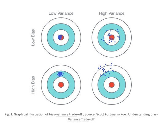
Bias
It is the difference between the model’s prediction and the real value. A model with high bias can cause an algorithm to miss the relevant relations between features and target outputs and oversimplifies the model. These models have a high error on training and test data (underfitting). eg. Linear regression is a simple model that may be prone to high bias if the problem is not linear.

Variance
It is the amount by which the prediction would change if we estimated it using a different training data set ( = sensitivity of the model to a new data point). A model with high variance does not generalize on data that it hasn’t seen before. As a result, such models perform very well on training data but has high error rates on test data (overfitting, i.e modeling the random noise in the training data, rather than the intended outputs). eg. Flexible methods may be prone to high variance.

Flexibility
It measures how closely the model fits the train data. A flexible method can decrease the bias but it will increase the variance (i.e. it is prone to overfitting). Eg. a NN with a large number of layers and neurons.

Cross-validation = rotation estimation
It is a model validation technique for assessing how the results of a statistical analysis will generalize to an independent data set. It give an estimation of the test MSE using the training data only. Some cross-validation techniques include K-fold cross-validation, Leave-One-Out cross-validation and stratified cross-validation.

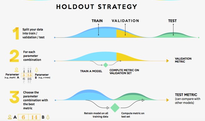
Hold-out validation

• Pros: Fully independent data; only needs to be run once so has lower computational costs.
• Cons: Performance evaluation is subject to higher variance given the smaller size of the data.

_^Source

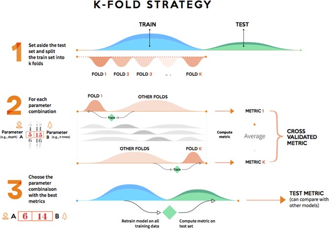
K-fold cross-validation

• Pros: Prone to less variation because it uses the entire training set.
• Cons: Higher computational costs; the model needs to be trained K times at the validation step (plus one more at the test step).

_^Source

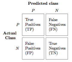
Confusion matrix = error matrix
It is a table used to visualise the performance of a classification model on a set of test data for which the true values are known. (True Positive, True Negative, False Positive, False Negative)

_^Source

Logistic regression
Simple supervised learning algorithm for classification problems. It predicts the probability of a class by fitting data to a logit function.

Linear Discriminant Analysis (LDA)
Classification algorithm that uses a linear combination of input features to predict the output class.

Quadratic discriminant analysis (QDA)
LDA with quadratic terms.

Classification and Regression Tree (CART) = Decision trees
Classification trees split the population into two or more homogeneous sets (or sub-populations) based on most significant splitter / differentiator in input variables.

Linear regression = Ordinary Least Squares (OLS)
Regression algorithm that fit a linear equation between independent variables Y and dependent variables X (e.g. Y = a*X + b). The coefficients are found using the method of the least squares.

Multiple regression
Linear regression with more than one dependent variable. (e.g. Y = aX1 + bX2 + c).

Polynomial regression
Regression with polynomial terms.

Generalized Linear Models (GLM)
They are generalisations of the linear regression algorithm. eg. Lasso, Ridge regression, ElasticNet

Regularization
It is the process of introducing additional information in order to solve an ill-posed problem or to prevent over-fitting. eg. L1 or L2 regularization

LASSO (Least Absolute Shrinkage and Selection Operator)
Linear regression with L1 regularization.

Ridge regression (= Tikhonov regularization = Tikhonov-Miller method = Phillips-Twomey method)
Linear regression with L2 regularization.

ElasticNet
Linear regression with both L1 and L2 regularization.

Generalised Additive Model (GAM)
Special case of GLM.

Support vector machines (SVM)
Supervised learning models used for classification or regression.

Naive Bayes
They are a family of simple probabilistic classifiers based on applying Bayes’ theorem with strong (naive) independence assumptions between the features.

Balanced Iterative Reducing and Clustering using Hierarchies (BIRCH)
It is an unsupervised machine learning algorithm used to perform hierarchical clustering over particularly large data-sets.

Ensembling = ensemble methods
They combine multiple learning algorithms to obtain better predictive performance than could be obtained from any of the constituent learning algorithms alone. Eg. bagging, boosting, random forest

Bagging = Bootstrap Aggregation
It is an ensemble algorithm used to improve the stability and accuracy of supervised learning algorithms. It decreases the variance of the predictions by increasing the size of the training set using combinations with repetitions.

Boosting
It is an ensemble meta-algorithm used to reduce the bias and the variance in supervised learning.

Autoregressive-moving-average (ARMA) and Autoregressive integrated moving average (ARIMA)
They are statistical models used for analyzing and forecasting time series data.

Density-based spatial clustering of applications with noise (DBSCAN)
It’s an unsupervised clustering algorithm that groups together points that are closely packed together, marking as outliers points that lie alone in low-density regions.

Probabilistic graphical model (PGM) = structured probabilistic model
It is a probabilistic model for which a graph expresses the conditional dependence structure between random variables. Eg. Bayesian network, Conditional random fields

Bayesian network = Bayes network = belief network = Bayesian model
They are a type of PGM that uses Bayesian inference for probability computations. Bayesian networks aim to model conditional dependence, and therefore causation, by representing conditional dependence by edges in a directed graph.

Probabilistic directed acyclic graphical model
It is a PGM that represents a set of random variables and their conditional dependencies via a Directed Acyclic Graph (DAG)

XGBoost
It is an optimized distributed gradient boosting library designed to be highly efficient, flexible and portable. XGBoost provides a parallel tree boosting (also known as GBDT, GBM) that solve many data science problems in a fast and accurate way.

Random Forest
It is an ensemble learning method used in a supervised learning context (classification or regression problems). It operates by constructing a multitude of decision trees at training time and outputting the class that is the mode of the classes (classification) or mean prediction (regression) of the individual trees.

Dimensionality reduction algorithms
They are unsupervised learning techniques to reduce the number of features in a data by extracting relevant information and disposing rest of data as noise. There are 2 main type of dimensionality reduction techniques: linear and non-linear.

Manifold learning
It is a subset of nonlinear dimensionality reduction methods. The aim is to extract newer and richer hidden knowledge from the original data.

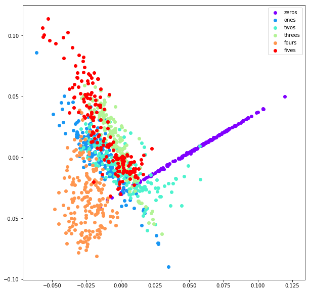
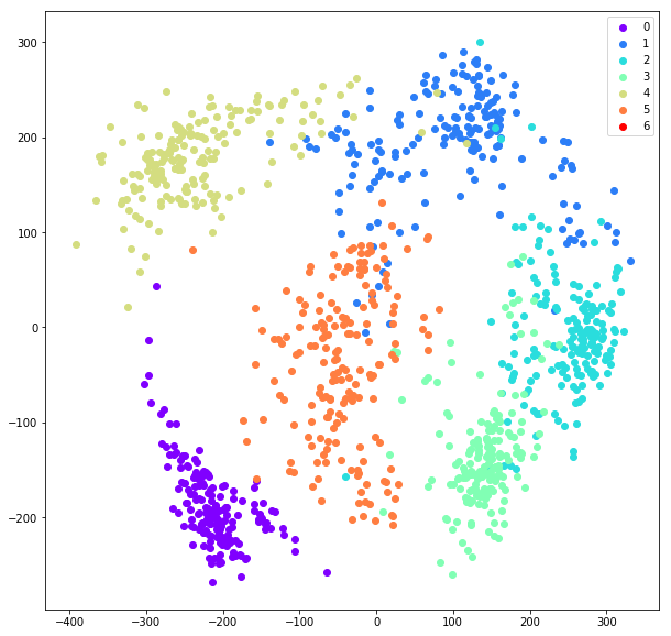
Principal Component Analysis (PCA)
It is a linear dimensionality reduction algorithm that reduce the original variables into a lower number of orthogonal - non correlated - synthesized variables called Principal Components (i.e. eigenvalues).
CONS: If the number of variables is large, it becomes hard to interpret the principal components. PCA is most suitable when variables have a linear relationship among them. Also, PCA is susceptible to big outliers. PCA was invented in 1901… there are more modern techniques out there. Some improvements of PCA are: robust PCA, kernel PCA and incremental PCA.

_^Source

Independent Component Analysis (ICA) = Blind Source Separation = Cocktail party problem
It is a linear dimension reduction method, which transforms the dataset into columns of independent components. It assumes that each sample of data is a mixture of independent components and it aims to find these independent components.
CONS: ICA cannot uncover non-linear relationships of the dataset. ICA does not say anything about the order of independent components or how many of them are relevant.

Multi-Dimension Scaling (MDS)
It is a distance-preserving manifold learning method.
CONS: MDS requires large computing power for calculating the dissimilarity matrix at every iteration. It is hard to embed the new data in MDS.

_^Source

Locally Linear Embedding (LLE)
It is a topology preserving manifold learning method.
CONS: LLE is sensitive to outliers and noise. Datasets have a varying density and it is not always possible to have a smooth manifold. In these cases, LLE gives a poor result. Some improvements of LLE are: Hessian LLE, Modified LLE, and LTSA.

_^Source

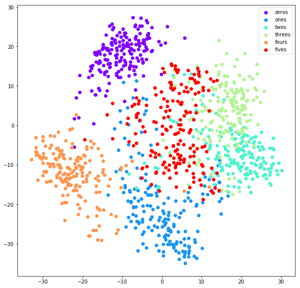
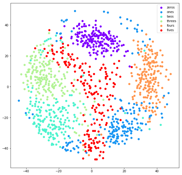
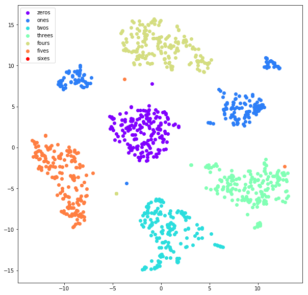
t-distributed Stochastic Neighbor Embedding (t-SNE)
It is a manifold learning technique that converts affinities of data points to probabilities.
CONS: When considering more than 2-3 dimensions, t-SNE has the tendency to get stuck in local optima like other gradient descent based algorithms. The basic t-SNE algorithm is slow due to nearest neighbor search queries. An improvement of t-SNE is Barnes-Hut-SNE.

_^Source

Isomap (= isometric mapping)
It is a manifold learning method based on the spectral theory which tries to preserve the geodesic distances in the lower dimension.
CONS: Isomap performs poorly when manifold is not well sampled and contains holes. As mentioned earlier neighborhood graph creation is tricky and slightly wrong parameters can produce bad results.

_^Source

Spectral Embedding
It is a manifold learning approach for calculating a non-linear embedding.

Self-organizing map (SOM) = self-organising feature map (SOFM)
It is an unsupervised learning technique for dimensionality reduction where a ANN is trained to produce a low-dimensional (typically two-dimensional), discretized representation of the input space of the training samples, called a map.

Local Outlier Factor (LOF)
It is an unsupervised learning algorithm for anomaly detection. It measures the local deviation of a given data point with respect to its neighbours.

4. Deep Learning

Artificial Neural Networks (ANN)
It’s a computational model based on the structure and functions of biological neural networks. They are used to estimate functions that can depend on a large number of inputs and are generally unknown.

Feedforward Neural Networks (FNN)
It is the simplest form of neural networks where a number of simple processing units (neurons) are organized in layers. Every neuron in a layer is connected with all the neurons in the previous layer. These connections are not all equal: each connection may have a different strength or weight. The weights on these connections encode the knowledge of a network. Eg. Single Layer Perceptron (SLP), Multi Layer Perceptron (MLP)

Perceptron
It is the simplest form of neural network.

Deep Neural Network
It is an artificial neural network with an input layer, an output layer and at least one hidden layer in between.

Backpropagation
It is the algorithm used for computing the gradient of the cost function in a neural network. It is used to adjust the weights and bias of a neural network during the training phase.

Gradient descent
It is an optimization algorithm used to minimize some function by iteratively moving in the direction of steepest descent as defined by the negative of the gradient. In machine learning, we use gradient descent to update the parameters (or weights and biases in the case of an ANN) of our model.

Stochastic Gradient Descent
It’s a less computationally expensive way of calculating the gradient’s slope than the Batch Gradient Descent method.

Neuron activation function
Relu (Rectified Linear Unit), Sigmoid, Softmax

Softmax
It is an activation function that turns numbers aka logits into probabilities that sum to one. It is used for multi-class classifiers.

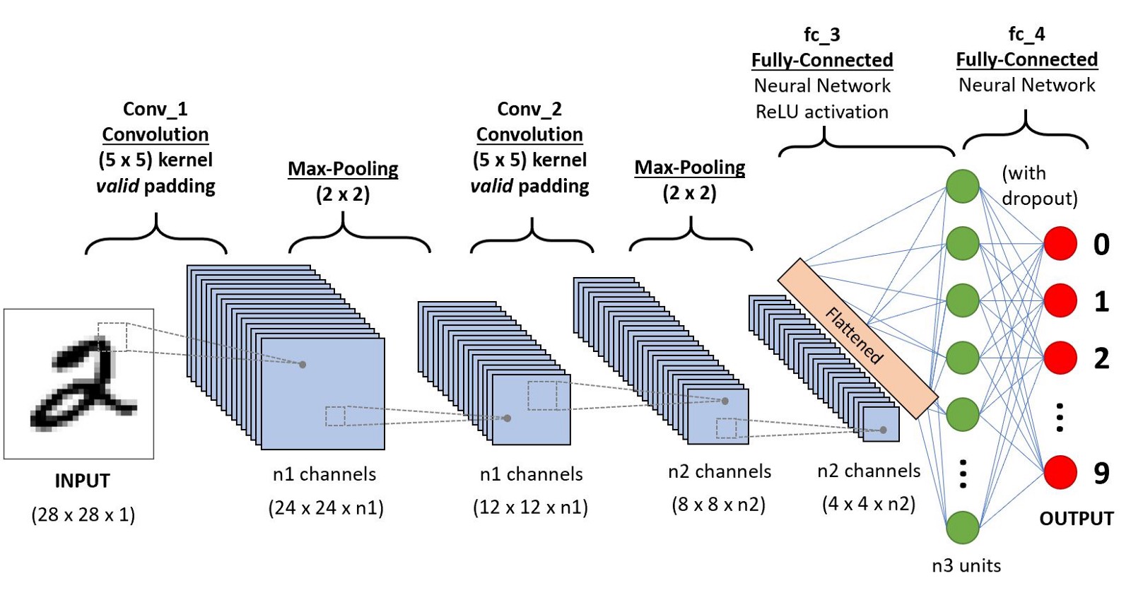
Convolutional Neural Network (CNN) = ConvNet
It is a deep neural network used for image recognition where the input neurons are replaced by a kernel convolution (i.e. a mask or filter applied to the image in order to extract important features such as edges).

_^Source

Famous examples of CNN architectures for image classification on the IMAGENET dataset

• LeNet (Yann LeCun, 1998)
• AlexNet (2012)
• ZFNet (2013)
• GoogleNet (2014)
• VGGNet (Visual Geometry Group, Oxford, 2014)
• VGG16
• VGG19
• ResNet

Image filters used in CNNs
Gaussian blur, Sobel edge detector, Canny edge detector

WaveNet
It is a deep NN for generating raw audio created by DeepMind. This netwrok is able to generate realistic-sounding human-like voices by sampling real human speech and directly modelling waveforms. The voices generated sound more natural than the traditional Text-to-Speech systems.

Residual Neural Network (ResNet)
It is a type of neural network that use short-cuts to jump over some layers (using gated recurrent units) in order to limit the vanishing gradient problem.

Vanishing gradient problem
It is a difficulty found in training artificial neural networks with gradient-based learning methods and backpropagation. The gradient of loss tends to get smaller and smaller as we move backwards in the network.

Autoencoder (AE) = autoassociator = Diabolo network
They are neural networks that aims to reconstruct their inputs as their outputs. The goal of an AE is to learn the underlying manifold or the feature space in the dataset (in order to reduce the dimensionality of the dataset).

Variational Auto-Encoder (VAE)
Instead of just learning a compressed representation of the data, VAE learn the parameters of a probability distribution representing the data.

Restricted Boltzmann Machine (RBM) (energy-based model)
It is a generative stochastic ANN that can learn a probability distribution over its set of inputs.

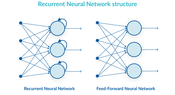
Recurrent Neural Network (RNN)
It is a neural network with feedback connections – unlike in a FNN – that is useful to identify patterns for data organised in time series. RNNs are characterised by a loop structure where the output from previous step are fed as input to the current step. They have a memory mechanism, which makes them suitable for applications where sequence is important such as in Natural Language Processing (e.g. speech recognition, handwriting recognition, chat bots), image captioning, self-driving cars, time series forecasting.

_^Source

Gated Recurrent Units (GRU)
It is an improvement of RNN that attempt to tackle the vanishing/exploding gradient problem by using a forget mechanism (up gate and reset gate).

Long Short-Term Memory network (LSTM)
It is a type of RNN that mitigate the vanishing / exploding gradient problem. It is a more sophisticated version of the GRU.

Attention mechanism
It’s an improvement for RNN and LSTM allowing them to focus on certain parts of the input sequence when predicting a certain part of the output sequence, enabling easier learning and of higher quality.

Skip connections
It consists in skipping some layers in a neural network architecture and feeding the output of one layer as the input to the next ones (as opposed to only the next one), typically 2 to 3 layers.

Residual blocks
It’s a block of layer composed of skip connections. They are used to make deeper networks easier to optimize, such as in ResNet.

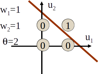
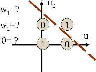
XOR problem
It is a classic problem in ANN research. It is the problem of using a neural network to predict the outputs of XOr (Exclusive Or) logic gates given two binary inputs. An XOr function should return a true value if the two inputs are not equal and a false value if they are equal.

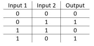
When solving a classification problem in 2D, the AND problem is linearly separable but the XOR problem is not.

_{^{AND problem – Source}}

_{^{XOR problem – Source}}

5. Machine learning software and tools

Machine Learning as a Service (MlaaS)
It is a range of cloud computing services that offer machine learning tools such as data pre-processing, model training, model evaluation (on-demand computing platform) (eg. Amazon Web Services (AWS) (EC2, S3, EMR), Microsoft AZURE, Google Cloud AI, IMB Watson, Google CoLab)

Deep learning libraries

• Tensorflow
• Pytorch
• Caffe
• Keras
• Theano

JMP
Software for statistical analysis.

SAS
It is a software suite for advanced analytics, multivariate analysis, business intelligence, data management, and predictive analytics.

SPSS
Software package used for statistical analysis.

Scala
It is a general-purpose programming language released in 2004 aimed to address criticisms of Java.

Julia
It is a high-level dynamic programming language designed to address the requirements of high-performance numerical and scientific computing while also being effective for general-purpose programming, web use or as a specification language.

Hardware for deep learning
CPU, GPU, TPU (Tensor Processing Unit)

Application-specific integrated circuit (ASIC)
It is a kind of integrated circuit that is specially built for a specific application or purpose. Eg. TPU

Hadoop
It is a distributed data infrastructure framework. It distributes large data sets across multiple nodes within a cluster.

Apache Hive
It is a system built on top of Hadoop to extract data from Hadoop using the same kind of methods used by traditional databases. It uses a SQL-like language called HiveQL.

Apache Pig
It is a high-level programming language used for analyzing large data sets with Hadoop.

Apache Mahout
It is a project of the Apache Software Foundation to produce free implementations of distributed or otherwise scalable machine learning

Kubernetes (= k8s)
It is an open-source container-orchestration system for automating application deployment, scaling, and management. For example, it can be used to manage Docker containers.

Relational vs non-relational databases (NoSQL)

• Relational databases represent and store data in tables and rows. They use SQL to query information. Eg. MySQL, PostgreSQL, SQLite3, Netezza, Oracle
• Non-relational databases store data without using a tabular structure, for example using collections of JSON documents. This database design is useful for very large sets of distributed data. Eg. MongoDB, Apache Cassandra

SQL (Structured Query Language, pronounced “sequel”)
It is a special-purpose programming language for relational database management systems.

JavaScript Object Notation (JSON)
It is an open-standard file format.

File formats used in machine learning
CSV, JSON, HDF5, Apache Parquet, AVRO, ORC, XML

Useful python libraries

• Numpy: an optimized library for numerical analysis, specifically: large, multi-dimensional arrays and matrices.
• Pandas: an optimized library for data analysis including dataframes inspired by R.
• Matplotlib: a plotting library that includes the pyplot interface which provides a MATLAB-like interface.
• Seaborn: a data visualization library based on Matplotlib
• Scipy: a library for scientific computing.
• Scikit-learn: machine learning library built on NumPy, SciPy, and Matplotlib.
• Pytorch: Deep learning library developed by Facebook.
• Tensorflow: Deep learning library developed by Google.
• OpenAI Gym: library that provides virtual environments and benchmark problems for reinforcement learning applications.

R (programming language)
It is a programming language for statistical computing and graphics. Some commons R libraries are:

• ggplot2: a plotting system for R
• dplyr (or plyr): a set of tools for efficiently manipulating datasets in R (supercedes plyr)
• ggally: a helper to ggplot2, which can combine plots into a plot matrix, includes a parallel coordinate plot function and a function for making a network plot
• ggpairs: another helper to ggplot2, a GGplot2 Matrix
• reshape2: “Flexibly reshape data: a reboot of the reshape package”, using melt and cast

Kaggle.com
It’s a web platform hosting data science competitions.

Famous data-sets

• MNIST: data set of handwritten digits
• IMAGENET: It a dataset of labelled images. Every year, the best classification algorithm compete during the ImageNet Large Scale Visual Recognition Challenge (ILSVRC).
• Tennessee Eastman Process: It’s a synthetic industrial process of a chemical plant. It is commonly used to study and evaluate the design of process monitoring and control techniques.

Design of Experiment (DoE) = Experimental design
It is the systematic process of choosing different parameters that can affect an experiment, in order to make results valid and significant. This may include deciding how many samples need to be collected, how different factors should be interleaved, being cognizant of ordering effects, etc.):

• A/B Testing (online experiment to determine whether one change causes another)
• Controlling variables and choosing good control and testing groups
• Sample Size and Power law
• Hypothesis Testing, test hypothesis
• Confidence level
• SMART experiments: Specific, Measurable, Actionable, Realistic, Timely

A/B testing = split testing
It is a marketing experiment wherein you “split” your audience to test a number of variations of a campaign and determine which performs better. In other words, you can show version A of a piece of marketing content (e.g. a website) to one half of your audience, and version B to another and identify which strategy performs the best.

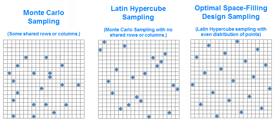
Monte Carlo Sampling (MCS) vs Latin Hypercube Sampling (LHS)

• Monte Carlo sampling generates a random sample of points for each uncertain input variable of a model. Because it relies on pure randomness, it can be inefficient. You might end up with some points clustered closely, while other intervals within the space get no samples.
• Latin Hypercube sampling is a statistical method for generating a near-random sample of parameter values from a multidimensional distribution. It is an efficient way to sample a search space with a minimum of evaluation (useful when evaluating the function takes a lot of time). LHS typically requires less samples and converges faster than Monte Carlo Simple Random Sampling (MCSRS) methods.

_^Source

Monte Carlo methods
They are a type of computational algorithm that rely on repeated random sampling to obtain numerical results. Their essential idea is using randomness to solve problems that might be deterministic in principle.

Markov Chain Monte Carlo (MCMC)
It is a method that draws samples randomly from a population in order to approximate the probability distribution of the population over a range of objects (eg. the height of men, the names of babies, etc…).

6. Machine learning steps

Exploratory Data Analysis (EDA)
It is the initial investigation of a data set so as to discover patterns, to spot anomalies, to test hypothesis and to check assumptions with the help of summary statistics and graphical representations (e.g. data visualisation)

Data cleaning = data filtering = data wrangling = data munging
It consists in collecting and cleaning data so it can be easily explored and analyzed later. Eg. convert “raw” data to a format that is easier to access and analyse, eliminate duplicated data.

Feature engineering = feature extraction
It is the process of using domain knowledge of the data to create new features. It is the process of transforming raw data into features that better represent the underlying problem to the predictive models, resulting in improved model accuracy on unseen data.

Feature selection = variable selection = attribute selection = variable subset selection
It is the process of selecting a subset of relevant features for use in model construction.

Feature learning = representation learning
It is a set of techniques that learn a feature: a transformation of raw data input to a representation that can be effectively exploited in machine learning tasks. This obviates manual feature engineering, which is otherwise necessary, and allows a machine to both learn at a specific task (using the features) and learn the features themselves: to learn how to learn.

Dimensionality reduction
It is the process of reducing the number of random variables under consideration.

Hyperparameter
They are the configuration variables of a machine learning algorithm. They are not directly related to the training data. Eg. number of hidden layers in an ANN, number of neurons in a layer, number of neighbors in KNN.

Hyperparameter optimization = hyperparameter tuning
It is the problem of choosing a set of optimal hyperparameters for a learning algorithm. eg. GridSearch, randomised parameter optimisation

Model selection
It is the process of choosing between different machine learning approaches – e.g. SVM, logistic regression, etc – or choosing between different hyperparameters or sets of features for the same machine learning approach. e.g. deciding between the polynomial degrees/complexities for linear regression.

Data integration
It involves combining data residing in different sources and providing users with a unified view of these data.

Model persistence
It’s the process of saving a trained machine learning model in a binary format in order to deploy it into production.

6. Statistics

6.1. Basics

Mean
Average value of a population.

Median
The value which divides the population in two half.

Mode
The most frequent value in a population.

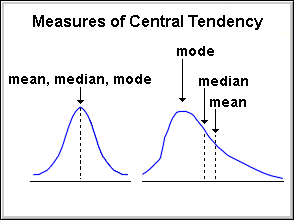
Central tendency
The value that describes the central position of a distribution (usually measured by the mean).

_^Source

Variance
The average of the squared differences from the mean.

Standard deviation
The square root of the variance. It measure of the dispersion of the data.

_^Source

Range
The difference in the maximum and minimum value in the population.

Sample statistic
Single measure of some attribute of a sample (e.g. mean, standard deviation, etc…).

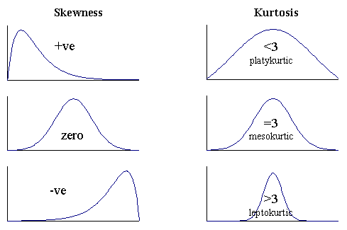
Skewness
It is a measure of the asymmetry of a distribution. Negatively skewed curve has a long left tail and vice versa.

Kurtosis
It is a measure of the “peaked-ness”. Distributions with higher peaks have positive kurtosis and vice-versa.

_^Source

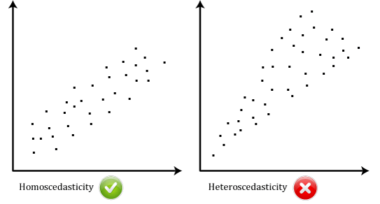
Homoscedasticity (= homogeneity of variance)
It describes a situation where all dependent variables exhibit equal levels of variance across the range of predictor variables, ie. the error term (that is, the “noise” or random disturbance in the relationship between the independent variables and the dependent variable) is the same across all values of the independent variables.

Heteroscedasticity
It refers to the situation where the size of the error term differs across values of an independent variable. Heteroscedasticity shows a ‘conic’ shape.

_^Source

Correlation
It is a measure of the linear relationship between independent variables.

Types of data distributions

• Normal (Gaussian) distribution
• Standard normal distribution
• Exponential/Poisson distribution
• Binomial distribution
• Chi-squared distribution
• F-distribution
• student T-distribution (= Cauchy distribution)

Box plot = whisker plot
It is a graphical representation of statistical data based on the minimum, first quartile, median, third quartile, and maximum.

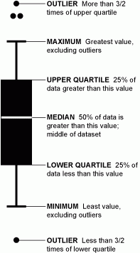
Quartiles
Values, which divide the population in 4 equal subsets (typically referred to as first quartile, second quartile and third quartile)

Inter-quartile range (IQR)
It is the difference in third quartile (Q3) and first quartile (Q1). By definition of quartiles, 50% of the population lies in the inter-quartile range.

Time series
It is a sequence of data points with associated time stamps.

6.2 Hypothesis testing

Null hypothesis
It refers to a general statement that there is no relationship between two measured phenomena, or no difference among groups. Eg. “there is no relationship between X and Y”

Rejecting the null hypothesis
It means that we believe that there is a relationship between two phenomena (e.g. that a potential treatment has a measurable effect).

P-value = observed significance level for the test hypothesis
It is the probability of finding the observed, or more extreme, results when the null hypothesis of a study question is true. If the p-value is equal to or smaller than the significance level (α, usually 5%), it suggests that the observed data are inconsistent with the assumption that the null hypothesis is true and thus that hypothesis must be rejected (but this does not automatically mean the alternative hypothesis can be accepted as true). A small p-value indicates that there is an association between the predictor and the response. For example, a p-value of 0.01 means there is only a 1% probability that the results from an experiment happened by chance. A predictor that has a low p-value is likely to be a meaningful addition to the model because changes in the predictor’s value are related to changes in the response variable.

Parametric vs non parametric tests
Parametric statistics are used to make inferences about population parameters. These inferences (from samples statistics to population parameters) are only valid if all assumptions (homogeneity of variance assumption or when the distribution is not perfectly normal) are met. It is possible to apply a quick fix to still use parametric tests. Otherwise, we use non parametric tests since they don’t assume a normal distribution.

Parametric statistics
It is a branch of statistics which assumes that the data have come from a type of probability distribution and makes inferences about the parameters of the distribution. Most well-known elementary statistical methods are parametric. Generally speaking, parametric methods make more assumptions than non-parametric methods. If those extra assumptions are correct, parametric methods can produce more accurate and precise estimates. They are said to have more statistical power. However, if assumptions are incorrect, parametric methods can be very misleading. For that reason they are often not considered robust. On the other hand, parametric formulae are often simpler to write down and faster to compute. In some cases, but not all, their simplicity makes up for their non-robustness, especially if care is taken to examine diagnostic statistics.

Nonparametric statistics
They are statistics that are not based on parametrized families of probability distributions. Unlike parametric statistics, nonparametric statistics make no assumptions about the probability distributions of the variables being assessed. The difference between parametric model and non-parametric model is that the former has a fixed number of parameters, while the latter grows the number of parameters with the amount of training data.

Parametric tests	Non-parametric tests
We know the distribution of the variables (eg normal)	We DON’T know the distribution of the variables (don’t require the assumption of sampling from a Gaussian population)
Big samples (>20)	Small samples (<20)
Compare mean and/or variance	Compare median and/or distribution
More powerful (ie. more accurate)	Less powerful (if the data is normally distributed)
Less robust	More robust

Statistical tests for significance

	Non correlated variables = independent = unpaired		Correlated variables = dependant = paired
	Normal distribution (parametric)	Don't know the distribution (non parametric)	Normal distribution (parametric)	Don't know the distribution (non parametric)
2 groups	Unpaired T-test	Mann-Whitney U test	Paired T-test	Paired Wilcoxon signed-rank test
More than 2 groups	ANOVA	Kruskall-Wallis	ANOVA	Friedman

Test statistic
It is a statistic (i.e. a quantity derived from the sample) used in statistical hypothesis testing.

ANOVA test = Analysis Of Variance
It’s a statistical model used to assess whether the average of more than two groups is statistically different. (if only 2 groups, use t-test or z-test)

Chi-Square Test
It is a test used to derive the statistical significance of relationship between 2 categorical variables.

• A probability of 0 indicates that both categorical variable are dependent.
• A probability of 1 shows that both variables are independent.
• A probability less than 0.05 indicates that the relationship between the variables is significant at 95% confidence.

Mann-Whitney U test (= Wilcoxon rank-sum test)
It is a non-parametric test of the null hypothesis that two samples come from the same population against an alternative hypothesis, especially that a particular population tends to have larger values than the other. It can be applied on unknown distributions contrary to the t-test which has to be applied only on normal distributions, and it is nearly as efficient as the t-test on normal distributions.

Wilcoxon signed-rank test
It is a non-parametric hypothesis test used when comparing two related samples, matched samples, or repeated measurements on a single sample to assess whether their population mean ranks differ (i.e. it is a paired difference test). It can be used as an alternative to the paired Student’s t-test, t-test for matched pairs, or the t-test for dependent samples when the population cannot be assumed to be normally distributed.

F-test
It refers to any statistical test in which the test statistic has an F-distribution under the null hypothesis. It is used for finding out whether there is any variance within the samples. F-test is the ratio of variance of two samples.

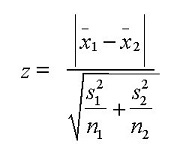
Z-test
It is a a test to assess whether mean of two groups are statistically different from each other or not (valid if n > 30 for both groups). A z-test is used for testing the mean of a population versus a standard, or comparing the means of two populations, with large (n > 30) samples whether you know the population’s standard deviation or not. It is also used for testing the proportion of some characteristic versus a standard proportion, or comparing the proportions of two populations (e.g. Comparing the average engineering salaries of men versus women, comparing the fraction defectives from 2 production lines.)

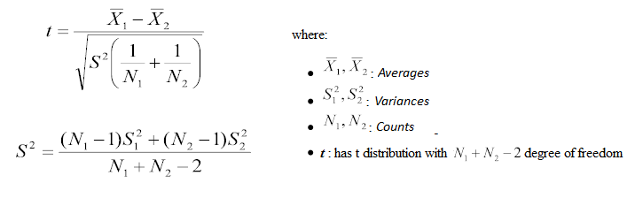
T-test
It is a test to assess whether mean of two groups are statistically different from each other or not (valid if n < 30 for both groups). A T-test refers to any statistical hypothesis test in which the test statistic follows a Student’s t-distribution if the null hypothesis is supported. It can be used to determine if two sets of data are significantly different from each other, and is most commonly applied when the test statistic would follow a normal distribution if the value of a scaling term in the test statistic were known. A T-test can determine if 2 features are related. It is used:

• to estimate a population parameter, i.e. population mean
• for hypothesis testing for population mean. Though, it can only be used when we are not aware of population standard deviation. If we know the population standard deviation, we will use Z-test.
• for finding out the difference in two population mean with the help of sample means.
• for testing the mean of one population against a standard or comparing the means of two populations if you do not know the population’s standard deviation and when you have a limited - sample (n < 30). If you know the population’s standard deviation, you may use a z-test. (For example, measuring the average diameter of shafts from a certain machine when you have a - small sample size).

Student’s t-distribution = t-distribution
It refers to any member of a family of continuous probability distributions that arises when estimating the mean of a normally distributed population in situations where the sample size and population standard deviation is unknown. Whereas a normal distribution describes a full population, t-distributions describe samples drawn from a full population; accordingly, the t-distribution for each sample size is different, and the larger the sample, the more the distribution resembles a normal distribution.

F statistic
It is a value obtained from an ANOVA test or a regression analysis. It can be used to find out if the means between two populations are significantly different.

R2 statistic
In regression models, R2 is a measure of the proportion of variability in Y that can be explained using X. i.e. it is a measure the linear relationship between X and Y.

Z table = standard normal table = unit normal table
It is a table containing the values of the cumulative distribution function of the normal distribution.

6.3 Statistical fields

Frequentist vs Bayesian statistics

• Frequentist statistics tests whether an event (hypothesis) occurs or not. It calculates the probability of an event in the long run of the experiment. A very common flaw found in frequentist approach i.e. dependence of the result of an experiment on the number of times the experiment is repeated.
• Bayesian statistics is a mathematical procedure that applies probabilities to statistical problems. It provides people the tools to update their beliefs in the evidence of new data.

Inferential statistics vs descriptive statistics vs predictive statistics

• Inferential statistics is the process of deducing properties about a population by studying a smaller sample of observations. Simple and inflexible methods such as Lasso or OLS are easier to interpret and to infer information.
• Descriptive statistics is solely concerned with properties of the observed data, and does not assume that the data came from a larger population. Descriptive statistics is the discipline of quantitatively describing the main features of a collection of information, or the quantitative description itself.
• Predictive statistics is the use of data, statistical algorithms and machine learning techniques to identify the likelihood of future outcomes based on historical data. The goal is to go beyond knowing what has happened to providing a best assessment of what will happen in the future.

Predictive inference
It is an approach to statistical inference that emphasizes the prediction of future observations based on past observations.

Causal modeling
It is the effort to go beyond simply discovering predictive relations among variables, to distinguish which variables causally influence others. e.g. a high white-blood-cell count can predict the existence of an infection, but it is the infection that causes the high white-cell count).

6.4. Metrics

Error metrics for regression Problems

• Mean Absolute Error
• Weighted Mean Absolute Error
• Mean Squared Error (MSE)
• Root Mean Squared Error
• Root Mean Squared Logarithmic Error (stub)

Error metrics for classification problems

• Logarithmic Loss
• Mean Consequential Error
• Mean Average Precision
• Multi Class Log Loss
• Hamming Loss
• Mean Utility
• Matthews Correlation Coefficient
• F1 score
• Precision
• Recall
• Confusion matrix

Error metrics for clustering problems

• Adjusted rand index
• Homogeneity
• V-measure

Error Metrics for probability distribution function

• Continuous ranked probability score

Metrics only sensitive to the order

• Area Under Curve (AUC)
• Gini
• Average Among Top P
• Average Precision (column-wise)
• Mean Average Precision (row-wise)
• Average Precision

Error Metrics for Retrieval Problems

• Normalized Discounted Cumulative Gain
• Mean Average Precision
• Mean F Score

Other and rarely used

• Levenshtein Distance
• Average Precision
• Absolute Error

Mean squared error (MSE) = mean squared deviation (MSD)
It measures the average of the squares of the errors – that is, the average squared difference between the estimated values and what is estimated. MSE is a risk function, corresponding to the expected value of the squared error loss.

Residual standard error (RSE)
In linear regression models, it is the average amount that the response will deviate from the regression line = lack of fit of the model eg: RSE = 3.26 means that if the model was correct (i.e. a and b known exactly in y = ax+b), any prediction would be off by about 3260 units on average.

Root Mean Square (RMS)
It is the square root of the mean square (the arithmetic mean of the squares of a set of numbers).

7. Famous people

Geoffrey Hinton
One of the pioneer of deep learning. He is known for his work on Boltzmann machines and capsules networks.

Yoshua Bengio
One of the pioneer of deep learning. He is known for his work on recurrent neural networks.

Yann LeCun
One of the pioneer of deep learning. He is known for his work on Convolutional Neural Networks and Backpropagation.

Andrew Ng
Very famous researcher in machine learning. Cofounder of Coursera and deeplearning.ai. Professor of Computer Science at Standford University. Cofounder of Google Brain and former chief scientist at Baidu.

Jürgen Schmidhuber
Famous computer scientist known for his work on LSTM.

Ian Goodfellow
He is known for his work in computer vision and Generative Adversarial Networks (GANs)

Andrej Karpathy
Director of AI at Tesla. Very active in the machine learning community..

Fei-Fei Li
Professor of Computer Science at Standford Univerisity. Iconic figure of the machine learning community.

Jeremy Howard
Researcher at Fast.ai

Richard S. Sutton
One of the founder of modern reinforcement learning.

Judea Pearl
He is known for his work on causality.

Other famous people
Rob Fergus, Nando de Freitas, Michael I Jordan, Terry Sejnowski, David M. Blei, Daphne Koller, Zoubin Ghahramani, Sebastian Thrun, Yaser S. Abu-Mostafa, Peter Norvig, Trevor Hastie, Robert Tibshirani, Anil K. Jain, Jitendra Malik, Vladimir Vapnik, Rachel Thomas