Reinforcement learning (RL) is a branch of machine learning that has gained a lot of momentum in the recent years. In this series, we will explain what is reinforcement learning and we will explore some implementation of the different types of RL techniques.
Definition
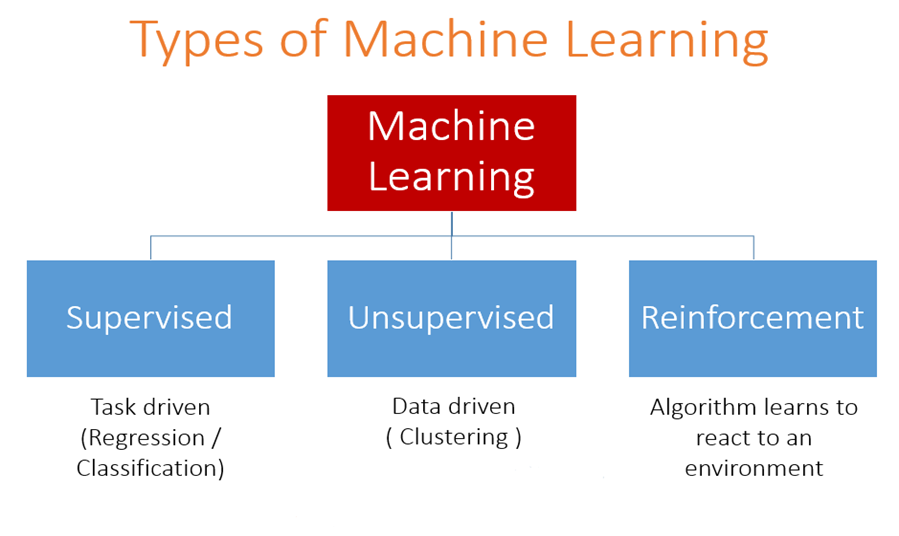
There are 3 main types of machine learning techniques: supervised learning, unsupervised learning and reinforcement learning. You may already be familiar with supervised learning, which consists in training a computer to make predictions give a set of labeled examples. On the other hand, unsupervised learning is attempting to find similarities in the data without using any labels. In reinforcement learning, the goal is to determine the actions that would maximize the total cumulative reward for a given problem.
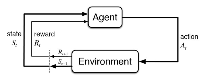
More formally, Reinforcement Learning (RL) is defined as “a type of machine learning technique that enables an agent to learn in an interactive environment by trial and error using feedback from its own actions and experiences.”[1]. The agent learns to make an informed decision by interrogating an unknown environment. The agent improves its decision-making abilities over time by maximizing a long-term reward through trial-and-error.
Here are some key definitions:
- Environment: Physical world in which the agent operates
- State: Current situation of the agent
- Reward: Feedback from the environment
- Policy: Method to map agent’s state to actions
- Value: Future reward that an agent would receive by taking an action in a particular state
Model free vs model based
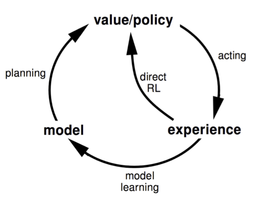
Model free = direct RL
Model free methods don’t build a model of the environment or reward; it just directly connects observations to actions (or values that are related to actions). The agent build directly a policy and/or a value function based on its observation of the environment.
Model based = indirect RL
The agent is given a model of the environment and uses this model to find the optimal actions. Model-based methods try to predict what the next observation and/or reward will be. Based on this prediction, the agent is trying to choose the best possible action to take, very often making such predictions multiple times to look more and more steps into the future.
Pros and cons
Usually pure model-based methods are used in deterministic environments, such as board games with strict rules. They require less samples so they also find nice applications in robotics. On the other hand, model-free methods are usually easier to train as it’s hard to build good models of complex environments with rich observations.
Value-based vs policy-based vs actor critic
Policy-based method
Policy-based methods are directly approximating the policy of the agent, that is, what actions the agent should carry out at every step. Policy is usually represented by probability distribution over the available actions. At each time step, the policy is updated but the value function is not stored (e.g. Policy gradient).
Value-based method
The agent calculates the value of every possible action and chooses the action with the best value i.e. the policy is not explicitly defined. (e.g. Q learning)
Actor critic method
Actor-critic methods store both the policy and the value function at each time step. It uses 2 neural networks:
- The critic measures how good the action taken is (value-based)
- The actor controls how our agent behaves (policy-based)
Pros and cons
Policy-based methods have better convergence properties. The problem with value-based methods is that they can have a big oscillation while training (high variability). This is because the choice of action may change dramatically for an arbitrarily small change in the estimated action values.
Episodic vs infinite horizon problems
Episodic problem
There is a starting state and a terminal state which defines an episode (e.g. Mario game, cartpole environment).
Infinite horizon
There is no terminal state. The agent has to learn how to choose the best actions and simultaneously interacts with the environment (e.g. stock trading).
Continuous vs discrete problems
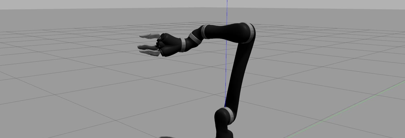
The state space and action space can be either discrete or continuous. Grid-world problems such as mazes have a discrete state and discrete action space. On the other hand, robotic arms have continuous state and action spaces.
Continuous problems are more difficult to solve. One solution could be to discretise a continuous space into bins. However, this may throw away valuable information regarding the geometry of the domain. It may also face the problem of the curse of dimensionality if the number of bins necessary is too large.
Deterministic vs stochastic policy
Deterministic policy
For each given state, a specific action will be executed (e.g. greedy policy). action = policy(state)
Stochastic policy
For each given state, there is a probability P that this action will be executed. It allows to make random exploratory decisions (e.g. Softmax policy) (action|state) = P(A=action|S=state)
Pseudo-deterministic policy
For each given state, there are two possibilities: either we execute a random action (exploration) or we execute the action following the target policy (exploitation). e.g. epsilon-greedy policy
Monte Carlo vs Temporal Difference
Monte Carlo methods
The agent waits until the end of the episode to look at the total cumulative reward.
Temporal difference (TD)
The agent update the maximum expected future reward at the end of each action / time step.
On-policy vs off-policy methods (TD learning)
Off-policy methods
Off-policy methods learn the optimal policy independently of the agent’s actions. They allow policy optimization on data obtained by a behavior policy different from the target policy being optimized. At every time step, 2 policies are updated:
- one that is learnt about and that becomes the optimal policy (target policy: exploitation)
- one that is more exploratory and is used to generate behavior (behaviour policy: exploration).
An off-policy agent does not always follow the target policy. e.g. Q-learning is an off-policy algorithm, since it updates the Q values (Bellman equation) without making any assumptions about the actual policy being followed (epsilon-greedy policy).
On-policy methods
On-policy approaches optimize the same policy that is used to make decisions during exploration. They learn the policy that is being executed during training, including the exploration steps. The on-policy agent can take into account the costs associated with exploration. (e.g. SARSA)
Pros and cons
Off-policy methods doesn’t depend on “freshness of data”. The agent can use very old data sampled from the environment several million steps ago, and this data will still be useful for learning. For this reason, off-policy methods can train on the previous large history of data (or even on human demonstrations) i.e. they can use a large experience replay buffer to make the data closer to being independent and identically distributed. They are more sample-efficient, however their training is less stable than on-policy approaches.
On-policy methods depend heavily on the training data to be sampled from to the current policy that is being learnt. Each time the policy is changed, even a little bit, we need to generate new samples. On-policy method require much more fresh data from the environment. They are usually less-sample efficient than off-policy methods, but they are more stable. They also scale well to high dimensional space problems.
Meta RL
Meta-learning (aka “learning to learn”) consists in training a model on various different tasks so that it can solve new learning tasks using only a small number of training samples Meta-RL is meta-learning on reinforcement learning tasks. After trained over a distribution of tasks, the agent is able to solve a new task by developing a new RL algorithm with its internal activity dynamics. Meta-RL distinguishes between learning to act in the environment (the reinforcement learning problem) and learning to learn (the meta-learning problem).
Challenges in reinforcement learning
Curse of dimensionality
It’s the combinatorial explosion of all possible actions to explore from all possible states.
Partial observability problem
In some problems (typically in a real world scenario), the agent may only have access to partial information on the state of the environment after performing an action. Some basic RL algorithm require full observability of the state.
Non-stationary environments
Some RL algorithms only work in quasi stationary environments where the dynamics change slowly. An RL method converging slowly will struggle to learn in non-stationary environments.
Exploration-exploitation dilemma
It’s the problem of finding the appropriate balance between exploration, where the agent gather more information and visit new states in the environment and exploitation, where the agent take the best decision given its current knowledge.
Temporal Credit Assignment Problem (CAP)
Given a long sequence of actions (e.g. sequence of moves in chess that lead to a win or loss), the CAP is the It is the problem of determining which actions were useful or useless in obtaining the final result (eg. win or loss in chess). It consists in assigning the relevant contribution to each actions.
Sparse reward
In some problems, the agent only receive a reward signal from the environment very infrequently, often only at the end of the episodes (eg when solving a maze). Some RL methods may only work in a dense reward setting.
Reward specification
RL problems require a reward to be defined and specified so that the agent can learn a policy for a given task. This reward function is often hand-crafted by human and may not be appropriate to learn to solve the task that was originally intended.
Sample efficiency
Some agents may require a lot of training iterations before learning successful policies.
Conclusion
We have just seen the definition of reinforcement learning and the main types of RL problems and methods. In the next post, I will talk about some common RL algorithms.




Leave a comment