Part 6 : Q learning for continuous state problems

In a previous post, we used Q-learning to solve simple grid-world problems such as a maze or the Taxi-v3 environment. For these type of problems, it was possible to use a Q-table composed of a finite number of rows corresponding to each possible state. However in most real-life problems, the number of possible states is infinite so it is virtually impossible to define a Q-table as in the previous post. A workaround consists in discretising the state space into buckets and use these buckets as an entry in the Q-table. I will illustrate this concept using the Cart-Pole environment from OpenAI Gym.

Cart-Pole environment

The Cart-Pole environment was described in a previous post. Basically, the agent must learn to balance an inverted pendulum by pushing a cart sliding on a rail towards the right or towards the left.

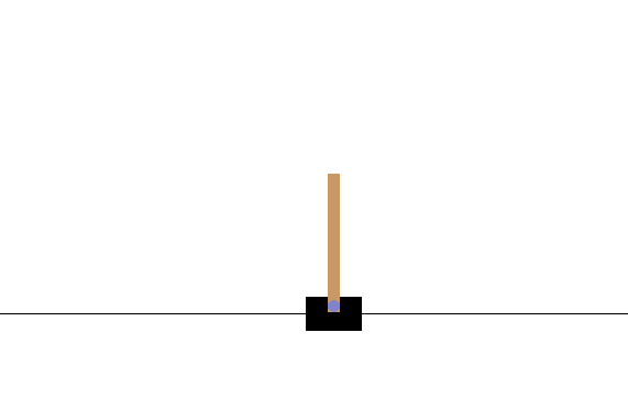
Let’s have a look at the environment’s action and state space.

import gym
import numpy as np
import math
import matplotlib.pyplot as plt

env = gym.make('CartPole-v0')

n_actions = env.action_space.n
n_states = env.observation_space.shape[0]
print("Action space size: ", n_actions)
print("State space size: ", n_states)

print('states high value: ', env.observation_space.high)
print('states low value: ', env.observation_space.low)

Action space size:  2
State space size:  4
states high value:  [4.8000002e+00 3.4028235e+38 4.1887903e-01 3.4028235e+38]
states low value:  [-4.8000002e+00 -3.4028235e+38 -4.1887903e-01 -3.4028235e+38]

The action space is discrete and can only take 2 values: push left (0) or push right (1). The state space is a continuous array of size 4 defined as follow: [cart position, cart velocity, pole angle, pole angular velocity].

Discretising the state space

In order to define the Q matrix, it is necessary to discretise each features in the state space into buckets (or bins).

# define the number of buckets for each state value (x, x', theta, theta')
buckets = (1, 1, 6, 12)     

# define upper and lower bounds for each state value
upper_bounds = [
        env.observation_space.high[0], 
        0.5, 
        env.observation_space.high[2], 
        math.radians(50)]

lower_bounds = [
        env.observation_space.low[0], 
        -0.5, 
        env.observation_space.low[2], 
        -math.radians(50)]

The optimal number of bucket for each state value (x, x’, theta, theta’) can be found by trial and error by attempting to maximise the sum of all the cumulative reward of all the episodes divided by the number of training episodes. Since we assign only one bucket to the cart position and velocity, it means that we ignore these 2 values.

Note that it is necessary to give finite bounds and reduce the range of the cart velocity and pole velocity at tip – i.e. [-0.5, +0.5] and [-50, +50], respectively – in order to be able to discretise.

Let’s now define the hyperparameters and some necessary functions.

# HYPERPARAMETERS
n_episodes = 1000           # Total train episodes
n_steps = 200               # Max steps per episode
min_alpha = 0.1             # learning rate
min_epsilon = 0.1           # exploration rate
gamma = 1                   # discount factor
ada_divisor = 25            # decay rate parameter for alpha and epsilon

# INITIALISE Q MATRIX
Q = np.zeros(buckets + (n_actions,)) 
print(np.shape(Q))

def discretize(obs):
    ''' discretise the continuous state into buckets ''' 
    ratios = [(obs[i] + abs(lower_bounds[i])) / (upper_bounds[i] - lower_bounds[i]) for i in range(len(obs))]
    new_obs = [int(round((buckets[i] - 1) * ratios[i])) for i in range(len(obs))]
    new_obs = [min(buckets[i] - 1, max(0, new_obs[i])) for i in range(len(obs))]
    return tuple(new_obs)

def epsilon_policy(state, epsilon):
    ''' choose an action using the epsilon policy '''
    exploration_exploitation_tradeoff = np.random.random()
    if exploration_exploitation_tradeoff <= epsilon:
        action = env.action_space.sample()  # exploration
    else:
        action = np.argmax(Q[state])   # exploitation
    return action

def greedy_policy(state):
    ''' choose an action using the greedy policy '''
    return np.argmax(Q[state])

def update_q(current_state, action, reward, new_state, alpha):
    ''' update the Q matrix with the Bellman equation '''
    Q[current_state][action] += alpha * (reward + gamma * np.max(Q[new_state]) - Q[current_state][action])

def get_epsilon(t):
    ''' decrease the exploration rate at each episode '''
    return max(min_epsilon, min(1, 1.0 - math.log10((t + 1) / ada_divisor)))

def get_alpha(t):
    ''' decrease the learning rate at each episode '''
    return max(min_alpha, min(1.0, 1.0 - math.log10((t + 1) / ada_divisor)))

The Q-matrix has now a dimension of (1 x 1 x 6 x 12 x 2). We can now train the agent as we have been doing it previously. The only difference is that we need to discretise the states received from the environment before passing them to the Q matrix.

# TRAINING PHASE
rewards = [] 

for episode in range(n_episodes):
    current_state = env.reset()
    current_state = discretize(current_state)

    alpha = get_alpha(episode)
    epsilon = get_epsilon(episode)

    episode_rewards = 0

    for t in range(n_steps):
        # env.render()
        action = epsilon_policy(current_state, epsilon)
        new_state, reward, done, _ = env.step(action)
        new_state = discretize(new_state)
        update_q(current_state, action, reward, new_state, alpha)
        current_state = new_state

        # increment the cumulative reward
        episode_rewards += reward

        # at the end of the episode
        if done:
            print('Episode:{}/{} finished with a total reward of: {}'.format(episode, n_episodes, episode_rewards))
            break

    # append the episode cumulative reward to the reward list
    rewards.append(episode_rewards)


# PLOT RESULTS
x = range(n_episodes)
plt.plot(x, rewards)
plt.xlabel('episode')
plt.ylabel('Training cumulative reward')
plt.savefig('Q_learning_CART.png', dpi=300)
plt.show()

# TEST PHASE
current_state = env.reset()
current_state = discretize(current_state)
episode_rewards = 0

for t in range(n_steps):
    env.render()
    action = greedy_policy(current_state)
    new_state, reward, done, _ = env.step(action)
    new_state = discretize(new_state)
    update_q(current_state, action, reward, new_state, alpha)
    current_state = new_state
    episode_rewards += reward

    # at the end of the episode
    if done:
        print('Test episode finished with a total reward of: {}'.format(episode_rewards))
        break
 
env.close()

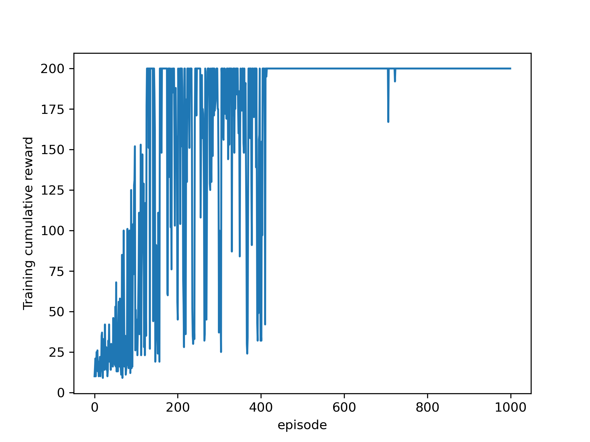
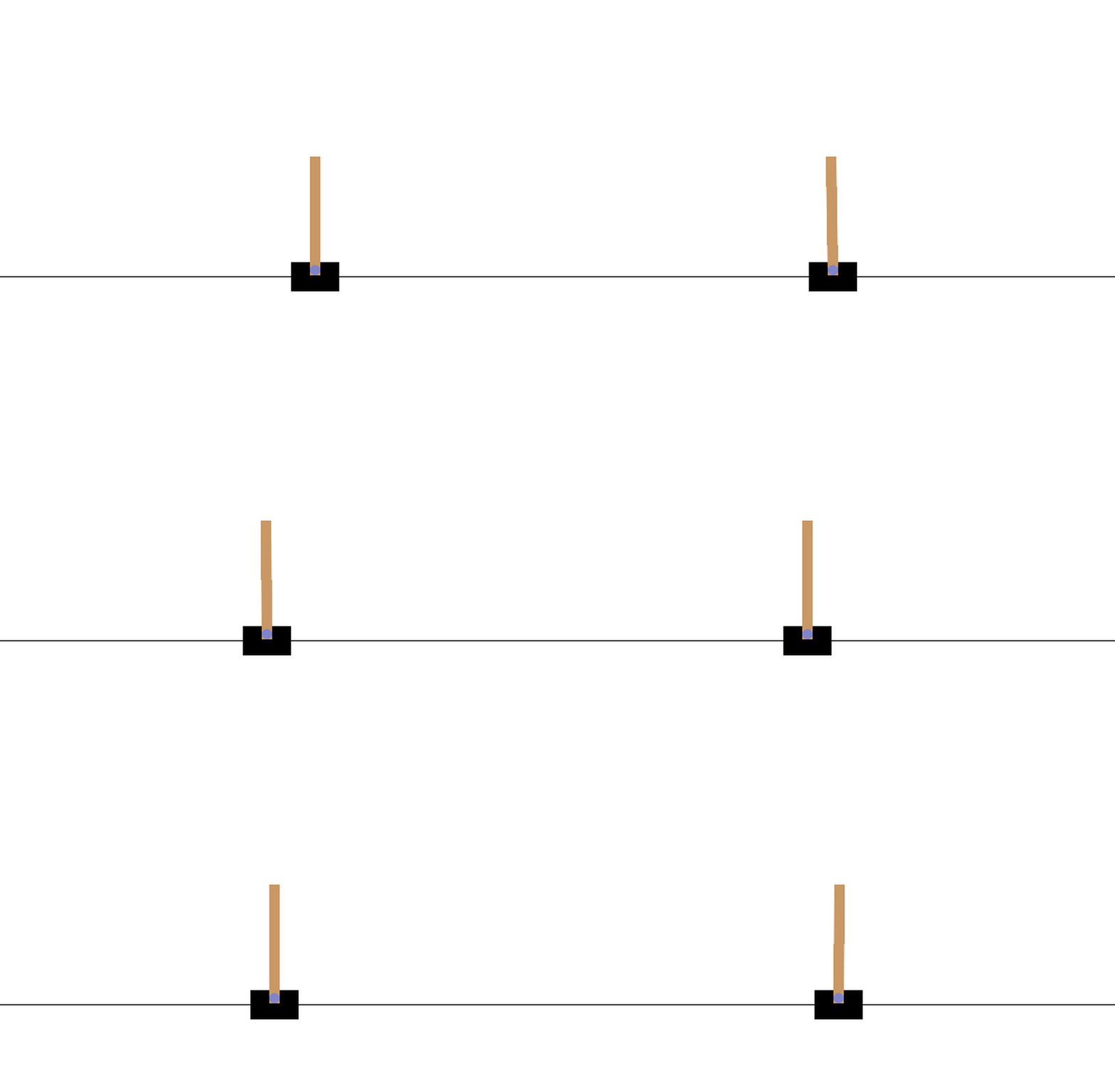
The training curve and the trained agent are shown below.

The full code can be found here.

Discretising the state and action space

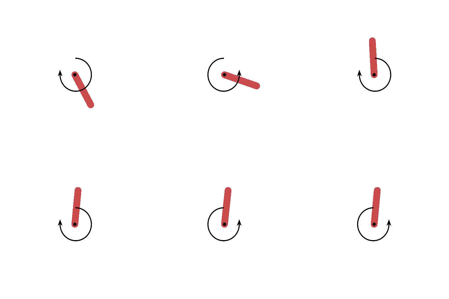
Some problems are characterised by continuous state and action space, such as the Pendulum-v1 environment. This environment simulates an inverted pendulum swingup problem, which is a classic problem in the control literature. In this version of the problem, the pendulum starts in a random position and the goal is to swing it up so it stays upright. In this environment, the state and action spaces are continuous. In order to apply Q-Learning, it is necessary to discretize the continuous state and action spaces into a number of buckets.

The full code can be found here.

The continuous action can be discretised into buckets as follows,

def discretize_action(action, lower_bounds, upper_bounds, buckets):
    ratios = (action + abs(lower_bounds)) / (upper_bounds - lower_bounds)
    new_action = int(np.round((buckets - 1) * ratios))
    new_action = min(buckets - 1, max(0, new_action))
    res = (new_action,)    # need to convert int to tuple
    return res

It is also necessary to convert the discretised action back to a float:

def convert_action_to_float(x):
    OldMax = action_buckets-1 
    OldMin = 0
    NewMax = 2
    NewMin = -2

    OldRange = (OldMax - OldMin)  
    NewRange = (NewMax - NewMin)  
    y = (((x - OldMin) * NewRange) / OldRange) + NewMin
    res = [y] # need to convert to a list to be readable by the step function
    return res

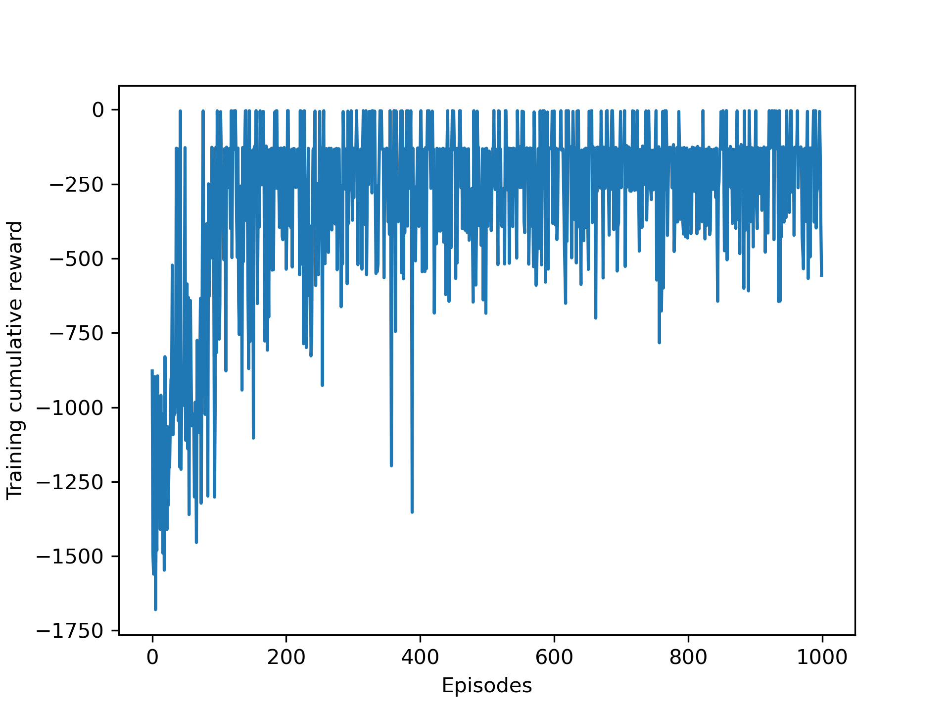
The training curve and the trained agent are shown below.

Limitations of the discretisation

It is relatively easy and efficient to discretise the state and action spaces for simple problems. However when the complexity increases, it is necessary to use smaller discretisation buckets and more of them in order to achieve a more accurate control of the agent and to receive a more precise information from the environment.

The problem with increasing the number of buckets is that the Q matrix becomes rapidly huge. For example an environment with 10,000 states and 1,000 actions per state would require a Q-table of 10 million cells! This present 2 problems:

• First, the amount of memory required to save and update that table would increase as the number of states increases and go beyond the memory of the computer.
• Second, the amount of time required to explore each state to create the required Q-table would be unrealistic.

This is known as the curse of dimensionality. In a future article, we will look at other strategies to deal with this problem, such as the famous Deep Q Network.