In previous posts, we have seen how Q learning works. However, we have also seen that it does not scale well as the problem complexity increases. That’s where Deep Q learning (DQN) comes to the rescue!
DQN architecture
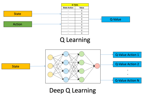
Deep Q learning basically consists in replacing the Q table by a deep neural network. There are some notable difference with standard Q learning however. In Q learning, the Q table was referencing a single Q value to each state-action pair. Instead a DQN only receives the current state as input and it outputs the Q values for each possible actions. This is essentially a regression problem. We only need to find the maximum Q value in order to find the best action. This is illustrated below.
A bit of theory
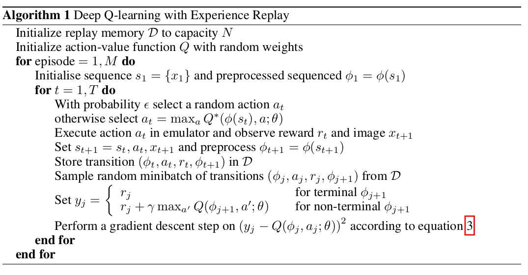
The idea behind DQN was published in 2013 by DeepMind. The pseudo-code of their DQN algorithm is shown below. Let’s have a look at it into more details.
Experience replay
In order to train the neural network, we first need to build some training data. This is known as Experience replay. The agent starts by taking random actions and stores its experience in memory. In practice, it means that the current state, action, reward, next state and termination status are appended to a list each time a new action is performed. We then randomly sample a minibatch of past experiences from the memory.
A neural network is built with so that it has an input and output layers equal to the size of the state and action space, respectively. In the Cart-Pole example, the state is described by 4 numbers (cart position, cart velocity, pole angle and pole velocity at tip) and there are 2 possible actions (push left (0) or push right (1)). So our network architecture can be defined as follows.
model = Sequential()
model.add(Dense(24, input_dim=n_states, activation='tanh'))
model.add(Dense(48, activation='tanh'))
model.add(Dense(n_actions, activation='linear'))
model.compile(loss='mse', optimizer=Adam(lr=alpha, decay=alpha_decay))
Now for each experience in the minibatch, we make an attempt to predict Q values from the current state using the neural network. In our case, we obtain 2 Q values corresponding to each action possible.
state = [ 0.0312954   1.02916599 -0.10072984 -1.59994526]
y_target = model.predict(state)
print(y_target)
[[14.886825 14.942211]]
We then update the Q value corresponding to the action taken in the past experience. For example, being in the current state, if the agent performed the action ‘left (0)’, we will update the first Q value and it it performed the action ‘right (1)’, we will update the second Q value. This Q value is updated either by the immediate reward if the episode is done, or by this value otherwise (Bellman equation):

Once we have updated all the Q values in the minibatch, we can build our training dataset with X being the states in the minibatch and y being the associated Q value vector. We can then use this dataset to fit the weights of the neural network.
The advantages of training the neural network on a randomly selection of the memory buffer (minibatch) are:
- it reduces correlation between experience thus creating an input data set stable enough for training and avoiding overfitting
- it increases the learning speed because we train on a smaller data set
The rest of the algorithm is similar to tabular Q learning as we saw in a previous post, i.e. at each time step,
- select an action using the epsilon-greedy policy
- execute the action and observe the next state and the reward
- store the experience in the memory
- update the current state by the next state
- update the Q values using experience replay
Let me see the code
The code can be found here.
Target network
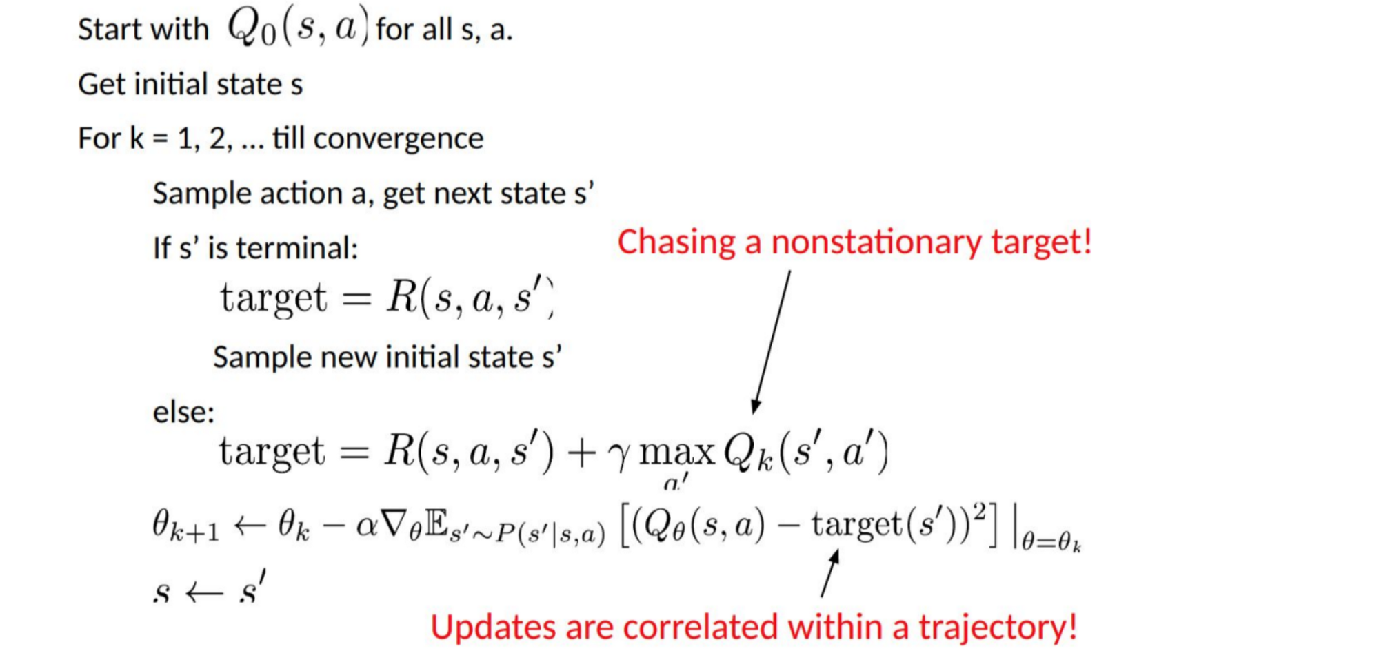
The problem with experience replay is that both the input and the target are constantly changing during training, making the training unstable. As shown below, the target values for Q depends on Q itself, we are chasing a non-stationary target.
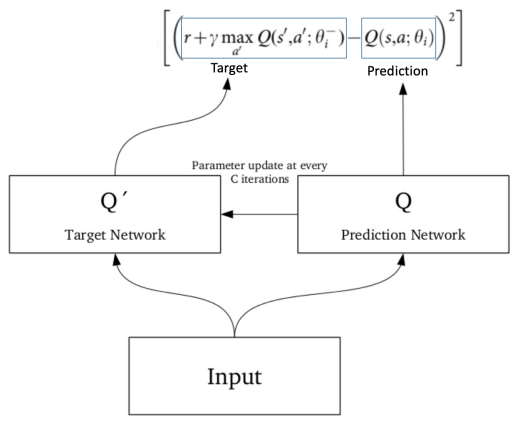
The solution consists in creating two deep networks with the same architecture: one with constant weights - the target network and one with variable parameters - the prediction network. The target network is used to estimate the target Q values and the prediction network is used to fit the network’s weight that minimise the loss. Every X steps (a large number eg. 100,000), these weights are synchronised with those of the target network to ensure stability of training. The objective is to fix the target Q values temporarily so we don’t have to chase a moving target.
Don’t reinvent the wheel: use RL libraries
The code above was simplified for clarity but it is far from being optimal. There are lots of deep reinforcement learning libraries out there that are written by teams of professional developers and optimised for efficiency. For example, keras-rl implement some recent deep reinforcement learning algorithms in Python (such as DQN, DDPG, NAF, SARSA, CEM) and integrates seamlessly with the deep learning library Keras.
An example using DQN from keras-rl to solve the cart-pole environment can be found here. The agent is trained much faster than using my handcrafted DQN example.


Leave a comment