Part 2 : The multi-layer perceptron

In the previous article, we learnt the theory behind the simplest neural network possible: the Single-Layer Perceptron. In this post, we will increase the complexity of the network by adding a hidden layer of neurons between the output and the input layer and build a Multi-Layer Perceptron (MLP). We will also introduce the Backpropagation algorithm.

Architecture of a MLP

We add a hidden layer of neurons between the output and the input layer, as follows:

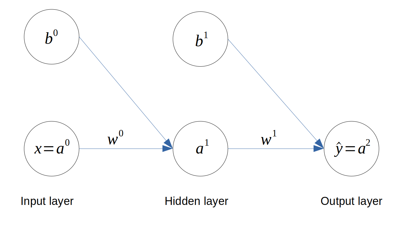_{^{Architecture of a Multi-Layer Perceptron}}

The layer number is shown in superscript for each variable.

Feedforward

We can now write the activation of each neuron as follows,

\[\begin{align*} \hat{y} = a^2 &= \sigma(z^2) \\ a^1 &= \sigma(z^1) \end{align*}\]

From the network architecture, we get:

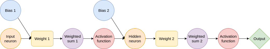
\[z^2 = a^1 w^1 + b^1 \\ z^1 = a^0 w^0 + b^0\]

The feedforward phase is illustrated below.

Backpropagation

The Mean-Square Error (MSE) cost function remains the same.

\[J = \frac{1}{m}\sum_{i=1}^{m}(a^2_i-y_i)^2\]

Last layer

Let’s apply Gradient Descent to the weight and bias of the last layer,

\[w^1 := w^1 - \alpha \frac{dJ}{dw^1} \\ b^1 := b^1 - \alpha \frac{dJ}{db^1}\]

The chain rule now becomes,

\[\frac{dJ}{dw^1} = \frac{dJ}{da^2} \frac{da^2}{dz^2} \frac{dz^2}{dw^1}\]

Isolating each terms, we have:

\[\begin{align*} \frac{dJ}{da^2} &= \frac{2}{m}(a^2-y) \\ \frac{da^2}{dz^2} &= \sigma'(z^2) \\ \frac{dz^2}{dw^1} &= a^1 \end{align*}\]

Similarly for the bias,

\[\frac{dJ}{db^1} = \frac{dJ}{da^2} \frac{da^2}{dz^2} \frac{dz^2}{db^1}\]

where \(\frac{dz^2}{db^1} = 1\)

The novelty here is that we also need to calculate the sensitivity of the cost function with respect to the activation of the previous layer \(a^1\). That’s why we call this method Backpropagation.

\[\frac{dJ}{da^1} = \frac{dJ}{da^2} \frac{da^2}{dz^2} \frac{dz^2}{da^1}\]

The only extra term we need to calculate is:

\[\frac{dz^2}{da^1} = w^1\]

First layer

We can now look at adjusting the weight and bias of the first layer by using the same idea.

Gradient descent for the weight in the first layer:

\[w^0 := w^0 - \alpha \frac{dJ}{dw^0}\]

Chain rule for the weight in the first layer:

\[\frac{dJ}{dw^0} = \frac{dJ}{da^1} \frac{da^1}{dz^1} \frac{dz^0}{dw^0}\]

where

\[\begin{align*} \frac{dJ}{da^1} &= \textrm{already calculated} \\ \frac{da^1}{dz^1} &= \sigma'(z^1) \\ \frac{dz^1}{dw^0} &= a^0 \end{align*}\]

Gradient descent for the bias in the first layer:

\[b^0 := b^0 - \alpha \frac{dJ}{db^0}\]

Chain rule for the bias in the first layer:

\[\frac{dJ}{db^0} = \frac{dJ}{da^1} \frac{da^1}{dz^1} \frac{dz^1}{db^{0}}\]

where \(\frac{dz^1}{db^0} = 1\)

Conclusion

We now have all the bits and pieces to update the weights and biases of all the layers. We won’t look at the implementation into Python code just yet because this example is a bit meaningless in practice since there is only one input neuron i.e. one feature. (So the best classification we can get in this case is input = output). In the next article, we will look at implementing a single-layer neural network with 3 input neurons.