
We have seen in a previous article that neural network with an input and one output layer are able to classify observations but only when the decision boundary is linear. In order to identify non-linear decision boundaries, we need to insert a fully-connected layer of neurons between the input and output layer. This type of network is called a Multi-layer Perceptron (MLP).
Data and architecture
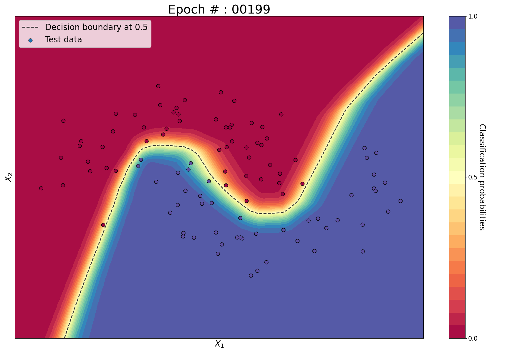
We consider a MLP to perform binary classification on a dataset of 500 observations with a non-linear decision boundary. Each observations has 2 features (X1 and X2). The red dots have the class 0 and the blue dots have the class 1.
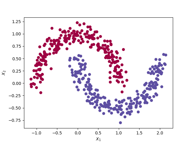 The moon dataset from the Sklearn library
Since we have 2 features, we need 2 input neurons. Since there are 2 classes to predict, we can use 1 output neuron (which can take the value 0 or 1). We choose to use 4 neurons in the hidden layer. The architecture of the network is as follows.
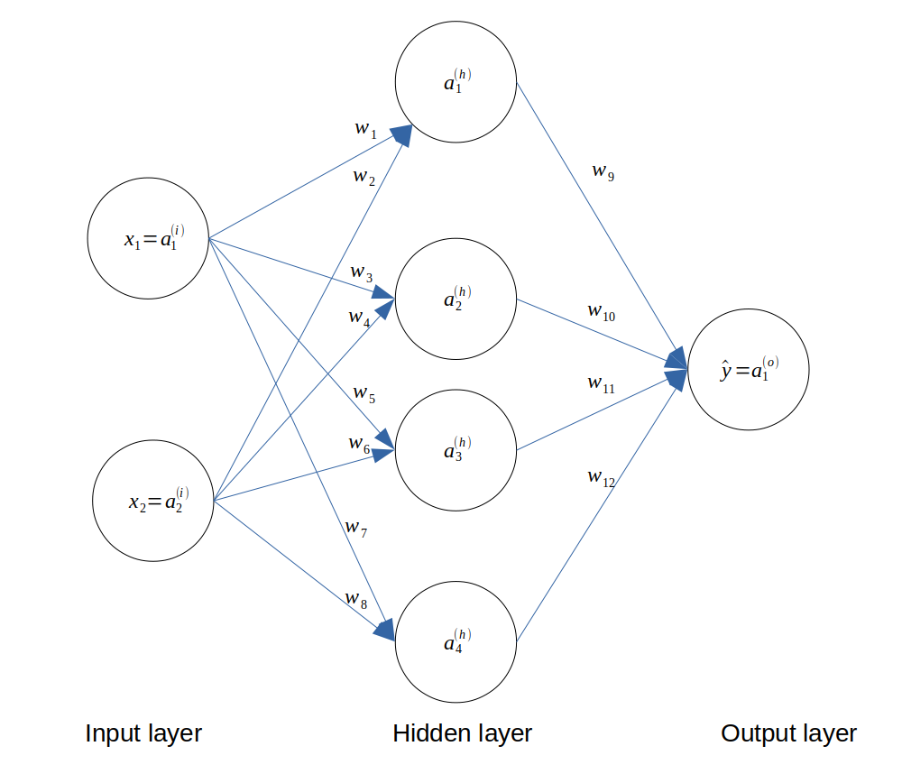 Architecture of the neural network
Note: we will not add the bias term for simplicity reasons.
Theory
The theory remains the same when we only had 2 layers (see this article). We just need to execute the feedforward and backpropagation passes in the following sequence:
- initialise the weights randomly
- feedforward pass between the input layer and the hidden layer to calculate \(a^{(h)}\)
- feedforward pass between the hidden layer and the output layer to calculate \(a^{(o)}\)
- backpropagation pass between the output layer and the hidden layer to calculate the gradient of the loss function with respect to the weights in the hidden layer \(\frac{\partial J}{\partial w^{(h)}}\)
- backpropagation pass between the hidden layer and the input layer to calculate the gradient of the loss function with respect to the weights in the input layer \(\frac{\partial J}{\partial w^{(i)}}\)
- update the weights using gradient descent
Python implementation
We start by importing some libraries and defining the Sigmoid function and its derivative.
from sklearn import datasets
import numpy as np
import matplotlib.pyplot as plt


def sigmoid(x):
    return 1/(1+np.exp(-x))

def sigmoid_der(x):
    return sigmoid(x) * (1-sigmoid (x))
We create a training and testing set using the convenient Scikit-Learn library.
np.random.seed(0)
X, y = datasets.make_moons(500, noise=0.10)
yy = y
y = y.reshape(500, 1)
X_test, y_test = datasets.make_moons(500, noise=0.10)
y_test = y_test.reshape(500, 1)
We initialise the weights randomly and we define the hyperparameters of the model.
wh = np.random.rand(len(X[0]), 4)
wo = np.random.rand(4, 1)
alpha = 0.5  # learning rate
nb_epoch = 5000
error_list = []
H = np.zeros((nb_epoch, 14))  # history
m = X.shape[0]  # number of observations
During the training phase, we perform feedforward and backpropagation steps using the MSE cost function, the chain rule and the gradient descent algorithm.
for epoch in range(nb_epoch):

    # 1. feedforward between input and hidden layer
    zh = np.dot(X, wh)
    ah = sigmoid(zh)

    # 2. feedforward between hidden and output layer
    zo = np.dot(ah, wo)
    ao = sigmoid(zo)

    # 3. cost function: MSE
    J = (1/m) * (ao - y)**2

    # 4. backpropagation between output and hidden layer
    dJ_dao = (2/m)*(ao-y)
    dao_dzo = sigmoid_der(zo)
    dzo_dwo = ah

    dJ_wo = np.dot(dzo_dwo.T, dJ_dao * dao_dzo)  # chain rule

    # 5. backpropagation between hidden and input layer
    dJ_dzo = dJ_dao * dao_dzo
    dzo_dah = wo
    dJ_dah = np.dot(dJ_dzo, dzo_dah.T)
    dah_dzh = sigmoid_der(zh)
    dzh_dwh = X

    dJ_wh = np.dot(dzh_dwh.T, dah_dzh * dJ_dah)  # chain rule

    # 6. update weights: gradient descent (only at the end)
    wh -= alpha * dJ_wh
    wo -= alpha * dJ_wo

    # 7. record history for plotting
    H[epoch, 0] = epoch
    H[epoch, 1] = J.sum()
    H[epoch, 2:10] = np.ravel(wh)
    H[epoch, 10:14] = np.ravel(wo)

    print("Epoch {}/{} | cost function: {}".format(epoch, nb_epoch, J.sum()))
We can plot the evolution of the cost function and weights with the number of iterations (epoch).
plt.plot(H[:, 0], H[:, 1])
plt.xlabel('Epoch #')
plt.ylabel('Training error')
plt.savefig('plots/2_J_vs_epoch.png')
plt.show()

plt.plot(H[:, 0], H[:, 2], label='$w_1$', marker='x', markevery=200)
plt.plot(H[:, 0], H[:, 3], label='$w_2$', marker='x', markevery=200)
plt.plot(H[:, 0], H[:, 4], label='$w_3$', marker='x', markevery=200)
plt.plot(H[:, 0], H[:, 5], label='$w_4$', marker='x', markevery=200)
plt.plot(H[:, 0], H[:, 6], label='$w_5$', marker='x', markevery=200)
plt.plot(H[:, 0], H[:, 7], label='$w_6$', marker='x', markevery=200)
plt.plot(H[:, 0], H[:, 8], label='$w_7$', marker='x', markevery=200)
plt.plot(H[:, 0], H[:, 9], label='$w_8$', marker='x', markevery=200)
plt.plot(H[:, 0], H[:, 10], label='$w_9$', marker='o', markevery=200)
plt.plot(H[:, 0], H[:, 11], label='$w_{10}$', marker='o', markevery=200)
plt.plot(H[:, 0], H[:, 12], label='$w_{11}$', marker='o', markevery=200)
plt.plot(H[:, 0], H[:, 13], label='$w_{12}$', marker='o', markevery=200)
plt.xlabel('Epoch #')
plt.ylabel('Weights')
plt.legend()
plt.savefig('plots/2_Weights_vs_epoch.png')
plt.show()
 MSE vs epoch
The training error (MSE) is decreasing with the number of iterations, which is a good sign.
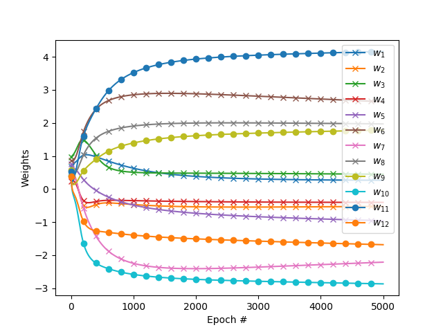 Weights vs epoch
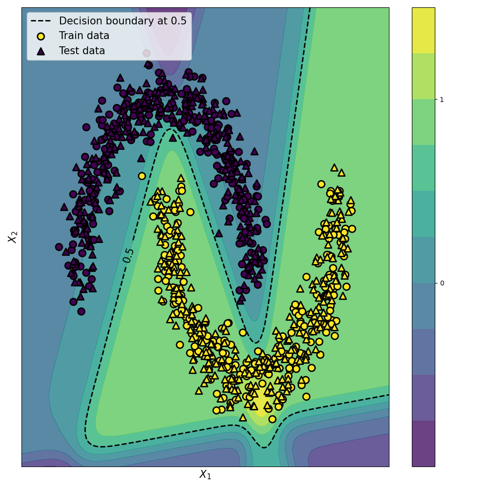
Finally, we test our network on the test set.
zh = np.dot(X_test, wh)
ah = sigmoid(zh)
zo = np.dot(ah, wo)
ao = sigmoid(zo)

y_hat = ao.round()
y_hat = y_hat.reshape(500,)

J_test = (1/m)*(ao - y_test)**2
print('Train error final: ', J.sum())
print('Test error final: ', J_test.sum())

plt.scatter(X[:, 0], X[:, 1], c=yy, cmap=plt.cm.Spectral, label="Train set")
plt.scatter(X_test[:, 0], X_test[:, 1], c=y_hat, cmap=plt.cm.Spectral, marker='x', label="Test set")
plt.xlabel('$X_1$')
plt.ylabel('$X_2$')
plt.legend()
plt.savefig('plots/2_test_vs_train.png')
plt.show()
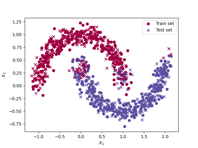 Train vs test set
We can see that most test data points have not been classified correctly but some were not. This could be improved by playing with the linearisation of the model. The final train MSE is 0.250 whereas the final test MSE is 0.254. The test error is higher than the final train error, which is expected.
You can find the code on my Github.
Conclusion
We performed binary classification on a problem with non-linear decision boundary using a Multi-Layer Perceptron. In the next article, we will see how to deal with multi-class classification problems.


Leave a comment