Part 5 : Multi-class classification with neural networks

In a previous article, we solved a binary classification on a problem with non-linear decision boundary using a Multi-Layer Perceptron. However, in many mase studies we need to classify observations in more than 2 classes. For example, the famous MNIST dataset is composed of images of handwritten digits and the problem consists in predicting the corresponding digit to each image. In this case, we need to construct a classifier that is capable of assigning values between 0 and 9 to each images, i.e. classify the observations into 10 classes. In this article, we will see how to deal with multi-class classification problems.

1. Problem description

Let’s consider a problem where we need to classify 2 dimensional data points into 3 classes: 0 (red), 1 (green) and 2 (blue).

2. Network architecture

Since our training data in 2 dimensional, we need 2 input neurons. We want to classify our data into 3 classes so we need 3 output neurons. We choose to have a hidden layer composed of 4 neurons. I did not draw the biaises for clarity reason but we will consider them in the derivation.

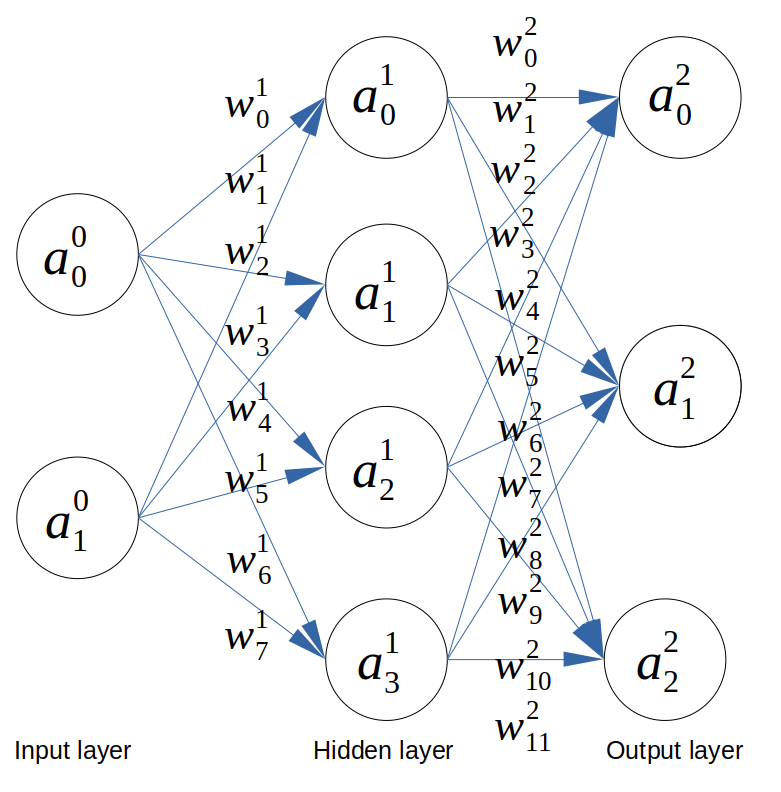_{^{Architecture of the neural network for multi-class classification}}

3. Feedforward

Based on the network architecture, we can derive the following:

\[\begin{align*} z^{1}_0 &= a^{0}_0 w^{1}_0 + a^{0}_1 w^{1}_1 + b^{1}_0\\ &\vdots\\ z^{2}_2 &= a^{1}_0 w^{2}_9 + a^{1}_1 w^{2}_{10} + a^{1}_2 w^{2}_{11} + a^{1}_3 w^{2}_{12} + b^{2}_2\\ \end{align*}\]

As you can see, it’s becoming pretty crammed and cumbersome to write. We will vectorise the equations as follows,

\[\begin{align*} Z^{1} &= W^{1}.A^{0} + B^{1} \\ Z^{2} &= W^{2}.A^{1} + B^{2} \end{align*}\]

Such as

\[\begin{bmatrix} z^{1}_0 \\ z^{1}_1 \\ z^{1}_2 \\ z^{1}_3 \end{bmatrix} = \begin{bmatrix} w^{1}_0 & w^{1}_1 \\ w^{1}_2 & w^{1}_3 \\ w^{1}_4 & w^{1}_5 \\ w^{1}_6 & w^{1}_7 \end{bmatrix} . \begin{bmatrix} a^{0}_0 \\ a^{0}_1 \end{bmatrix} + \begin{bmatrix} b^{1}_0 \\ b^{1}_1 \\ b^{1}_2 \\ b^{1}_3 \end{bmatrix}\]

and

\[\begin{bmatrix} z^{2}_0 \\ z^{2}_1 \\ z^{2}_2 \end{bmatrix} = \begin{bmatrix} w^{2}_0 & w^{2}_1 & w^{2}_2 & w^{2}_3 \\ w^{2}_4 & w^{2}_5 & w^{2}_6 & w^{2}_7 \\ w^{2}_8 & w^{2}_9 & w^{2}_{10} & w^{2}_{11} \end{bmatrix} . \begin{bmatrix} a^{1}_0 \\ a^{1}_1 \\ a^{1}_2 \\ a^{1}_3 \end{bmatrix} + \begin{bmatrix} b^{2}_0 \\ b^{2}_1 \\ b^{2}_2 \end{bmatrix}\]

4. Activation function

Since we are now using a vectorised notation, it becomes more convenient to use the Softmax function instead of the Sigmoid as activation function. The Softmax function takes a vector as input and produces another vector of the same length as output. This is why it is used in multi-class classification networks. It can be expressed as:

\[\theta(Z) = \frac{e^{Z}}{\sum_{j=1}^{k} e^{z_j}}\]

where \(Z = (z_1 ... z_k)\)

This function squashes the input vector to values between 0 and 1 where the sum is equal to 1. For example,

\[\theta \left( \begin{bmatrix} 1 \\ 2 \\ 3 \end{bmatrix} \right) = \begin{bmatrix} 0.09 \\ 0.24 \\ 0.67 \end{bmatrix}\]

In our multi-classification case study, we apply the Softmax function to the output layer only. We will still use the Sigmoid for the hidden layer.

\[\begin{align*} \hat{Y} = A^2 &= \theta(Z^2) \\ A^1 &= \sigma(Z^1) \end{align*}\]

5. Cost function

Instead of using the Mean Square Error (MSE) cost function, we will now use the Cross-Entropy function to minimise the loss.

\[H(Y, \hat{Y}) = - \sum_{i} y_i \log{\hat{y_i}}\]

This function is more convenient to use with the Softmax activation function. This function is also more efficient than MSE for multi-class classification problems.

6. Backpropagation

6.1. Ouput layer

We apply the Gradient Descent algorithm to the weights and biases of the last layer.

\[W^2 := W^2 - \alpha \frac{\partial H}{\partial W^2} \\ B^2 := B^2 - \alpha \frac{\partial H}{\partial B^2}\]

The chain rule gives:

\[\frac{\partial H}{\partial W^2} = \frac{\partial H}{\partial A^2} \frac{\partial A^2}{\partial Z^2} \frac{\partial Z^2}{\partial W^2} \\ \frac{\partial H}{\partial B^2} = \frac{\partial H}{\partial A^2} \frac{\partial A^2}{\partial Z^2} \frac{\partial Z^2}{\partial B^2}\]

The derivation of the cross-entropy function and the softmax function is quite complex. It can be shown that:

\[\frac{\partial H}{\partial A^2} \frac{\partial A^2}{\partial Z^2} = \hat{Y} - Y = \Delta^2\]

We also have:

\[\frac{\partial Z^2}{\partial W^2} = A^1 \\ \frac{\partial Z^2}{\partial B^2} = 1\]

Finally, we get the following update:

\[W^2 := W^2 - \alpha A^1 \Delta^2 \\ B^2 := B^2 - \alpha \Delta^2\]

6.2. Hidden layer

We apply the same principle to the hidden layer but we use the Sigmoid instead of the Softmax activation function.

The Gradient Descent algorithm gives:

\[W^1 := W^1 - \alpha \frac{\partial H}{\partial W^1} \\ B^1 := B^1 - \alpha \frac{\partial H}{\partial B^1}\]

The chain rule gives:

\[\frac{\partial H}{\partial W^1} = \frac{\partial H}{\partial A^1} \frac{\partial A^1}{\partial Z^1} \frac{\partial Z^1}{\partial W^1} \\ \frac{\partial H}{\partial B^1} = \frac{\partial H}{\partial A^1} \frac{\partial A^1}{\partial Z^1} \frac{\partial Z^1}{\partial B^1}\]

We apply the chain rule again:

\[\frac{\partial H}{\partial A^1} = \frac{\partial H}{\partial A^2} \frac{\partial A^2}{\partial Z^2} \frac{\partial Z^2}{\partial A^1} = \Delta^2 W^2\]

We have

\[\frac{\partial A^1}{\partial Z^1} = \sigma'(Z^1) = \sigma(Z^1)(1 - \sigma(Z^1)) = A^1 (1-A^1)\]

and

\[\frac{\partial Z^1}{\partial W^1} = A^0 = X\]

and

\[\frac{\partial Z^1}{\partial B^1} = 1\]

We get the following:

\[\frac{\partial H}{\partial W^1} = \Delta^2 W^2 A^1 (1-A^1) X \\ \frac{\partial H}{\partial B^1} = \Delta^2 W^2 A^1 (1-A^1)\]

Finally, the update of the hidden layer is

\[W^1 := W^1 - \alpha X \Delta^1 \\ B^1 := B^1 - \alpha \Delta^1\]

where \(\Delta^1 = \Delta^2 W^2 A^1 (1-A^1)\)

As a reminder, here is the meaning of each terms:

• \(Y\) : output labels (vector)
• \(X = A^0\) : input features (vector)
• \(A^1\) : activation of the hidden layer (vector)
• \(\hat{Y} = A^2\) : predicted output (vector)
• \(W^1\) : weights of the hidden layer (matrix)
• \(W^2\) : weights of the output layer (matrix)
• \(B^1\) : biases of the hidden layer (vector)
• \(B^2\) : biases of the output layer (vector)
• \(Z^1\) : input values of the neurons in the hidden layer (vector)
• \(Z^2\) : input values of the neurons in the output layer (vector)
• \(\sigma\) : Sigmoid function
• \(\theta\) : Softmax function
• \(H\) : Cross-entropy function
• \(\alpha\) : Learning rate

That’s enough maths for now, let put this in application!

Implementation

We start by importing some libraries and defining the Sigmoid, Softmax and Cross-entropy functions.

import numpy as np
import matplotlib.pyplot as plt

def sigmoid(x):
    return 1 / (1 + np.exp(-x))

def softmax(A):
    expA = np.exp(A)
    return expA / expA.sum(axis=1, keepdims=True)

def cost_function(y, yhat):
    """ Cross-entropy cost function (y and yhat are arrays) """
    return np.sum(-Y * np.log(yhat))

We create a train and test set. Each dataset is composed of 1500 observations clustered in 3 clouds of 500 observations each.

In our problem, we have 3 classes, which is why we built our network architecture with an output layer composed of 3 neurons corresponding to each class. We want the model to output an array of size 3 where one value is 1 while all the others remain at 0. For this reason, we convert the output vector

For multi-class classification problems, we need to define the output label as a one-hot encoded vector since our output layer will have three nodes and each node will correspond to one output class. We want that when an output is predicted, the value of the corresponding node should be 1 while the remaining nodes should have a value of 0. For that, we need three values for the output label for each record. This is why we need to create a one-hot encoded output array. In our case, the output array has 1 at index 0 for the first 500 observations, 1 at index 1 for next 500 observations and 1 at index 2 for the last 500 observations.

def create_dataset(seed_nb):
    """ 
    Create dataset of 1500 observations clustered in 3 Gaussian clouds.
    Each observation has two features. The data is randomly generated based on the seed seed_nb.
    """
    np.random.seed(seed_nb)
    # generate three Gaussian clouds each holding 500 points
    X1 = np.random.randn(500, 2) + np.array([0, -2])   # (500 X 2)
    X2 = np.random.randn(500, 2) + np.array([2, 2])    # (500 X 2)
    X3 = np.random.randn(500, 2) + np.array([-2, 2])   # (500 X 2)

    # put them all in a big matrix
    X = np.vstack([X1, X2, X3])  # (1500 X 2)

    # generate the one-hot-encodings output array
    labels = np.array([0]*500 + [1]*500 + [2]*500)  # (1500 X 1)
    Y = np.zeros((1500, 3))
    for i in range(1500):
        Y[i, labels[i]] = 1    # (1500 X 3)

    return X, Y

# Create train and test data
X, Y = create_dataset(seed_nb=4526)
X_test, Y_test = create_dataset(seed_nb=7516)

We define the hyperparameters of the model and initialise the weights and biases randomly.

alpha = 10e-6
samples = X.shape[0] # 1500 samples
features = X.shape[1] # 2 features
hidden_nodes = 4
classes = 3
nb_epoch = 10000

W1 = np.random.randn(features, hidden_nodes)  # (2 X 5)
b1 = np.random.randn(hidden_nodes)            # (5 X 1)
W2 = np.random.randn(hidden_nodes, classes)   # (5 X 3)
b2 = np.random.randn(classes)                 # (3 X 1)

During the training phase, we perform the feedforward and Backpropagation steps using the Sigmoid, Softmax and Cross-entropy functions and the equations derived previously.

costs = []

for epoch in range(nb_epoch):
    # Feedforward
    ## Layer 1
    Z1 = X.dot(W1) + b1  # (1500 X 5)
    A1 = sigmoid(Z1)  # (1500 X 5)

    ## Layer 2
    Z2 = A1.dot(W2) + b2 # (1500 X 3)
    A2 = softmax(Z2) # (1500 X 3)

    # cost function: cross-entropy
    J = cost_function(Y, A2)
    costs.append(J)

    # Backpropagation
    delta2 = A2 - Y              # (1500 X 3)
    delta1 = (delta2).dot(W2.T) * A1 * (1 - A1)    # (1500 X 5)

    # Layer 2
    W2 -= alpha * A1.T.dot(delta2)
    b2 -= alpha * (delta2).sum(axis=0)

    # Layer 1
    W1 -= alpha * X.T.dot(delta1)
    b1 -= alpha * (delta1).sum(axis=0)

    print("Epoch {}/{} | cost function: {}".format(epoch, nb_epoch, J))

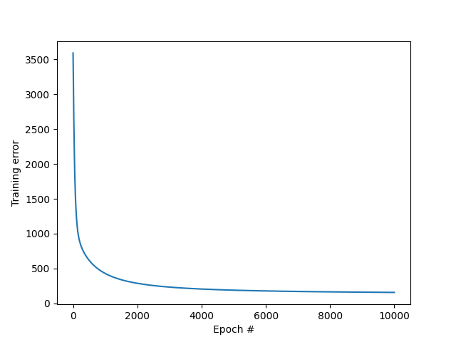
We can plot the evolution of the cost function with the number of epochs.

plt.plot(costs)
plt.xlabel('Epoch #')
plt.ylabel('Training error')
plt.savefig('plots/3_J_vs_epoch.png')
plt.show()

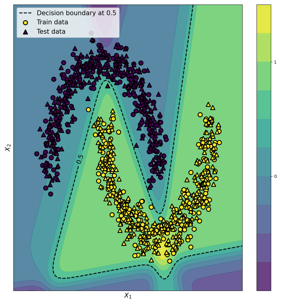
Finally, we test the model on unseen data.

# Feedforward
Z1 = X_test.dot(W1) + b1  # (1500 X 5)
A1 = sigmoid(Z1)  # (1500 X 5)

Z2 = A1.dot(W2) + b2 # (1500 X 3)
A2 = softmax(Z2) # (1500 X 3)

Y_hat = A2.round()

# calculate test error
J_test = cost_function(Y_test, A2)
print('Train error final: ', J)
print('Test error final: ', J_test)

plt.scatter(X[:,0], X[:,1], c=Y, cmap=plt.cm.rainbow, label="Train set") 
plt.scatter(X_test[:,0], X_test[:,1], c=Y_hat, cmap=plt.cm.rainbow, marker='x', label="Test set")
plt.xlabel('$X_1$')
plt.ylabel('$X_2$')
plt.legend()
plt.savefig('plots/3_test_vs_train.png')
plt.show()

You can find the code on my Github.

Conclusion

We successfully implemented a neural network that can classify observations into three classes.