Part 7 : Non-linear classification with Keras

We have seen in a previous post that it is much more convenient to use Deep Learning frameworks (such as Pytorch) than pure Numpy to build neural networks. In this post, we will build a neural network using another Deep Learning framework : Keras. Keras is a high-level neural network library that runs on top of TensorFlow. Keras is more user-friendly and offers a simple, concise, readable way to build neural networks than its famous counterparts, Pytorch and Tensorflow. However, since it’s written in Python, it is much slower and has a lower performance than Pytorch and Tensorflow. It is not recommended to use it in a production environment. The code in this post was adapted from this repository.

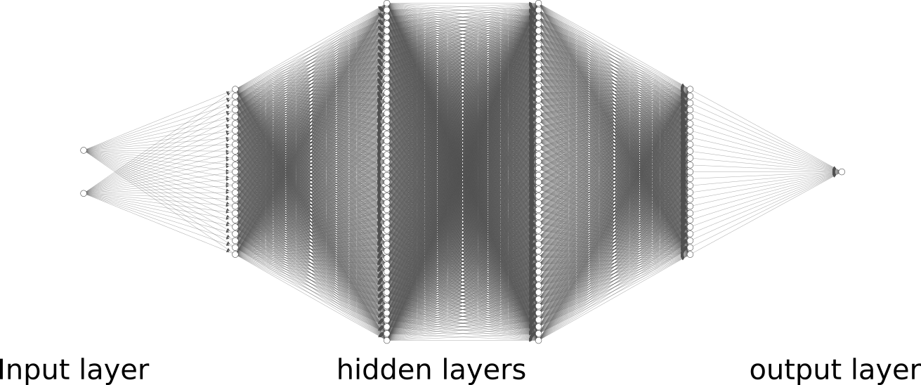
Network architecture

We will consider here a deeper architecture than in the previous post:

• 1 input layer of 2 neurons (since the observations are composed of 2 features)
• 1 hidden layer of 25 neurons
• 1 hidden layer of 50 neurons
• 1 hidden layer of 50 neurons
• 1 hidden layer of 25 neurons
• 1 output layer of 1 neuron (since we want to perform binary classification)

_{^{Network architecture}}

As you can see, it is much more complex and we can no longer derive the equations manually. This is when Keras will come handy.

Implementation

We start by importing the required libraries.

import numpy as np
from sklearn.datasets import make_moons
from sklearn.model_selection import train_test_split
from sklearn.metrics import accuracy_score
import matplotlib.pyplot as plt
from matplotlib import cm
import keras
from keras.models import Sequential
from keras.layers import Dense

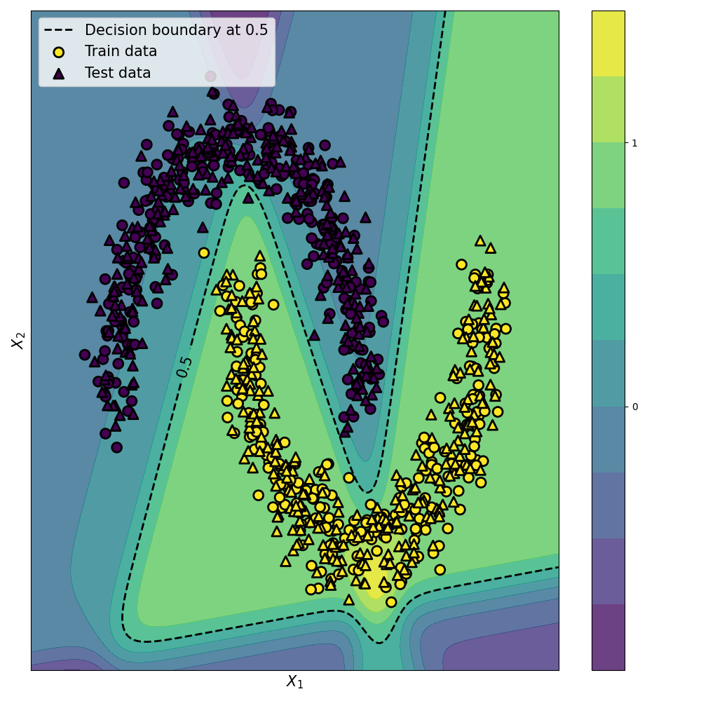
We consider the Moon dataset from Scikit-learn with 1000 observations made of 2 features.

X, y = make_moons(n_samples=1000, noise=0.2, random_state=100)
X_train, X_test, y_train, y_test = train_test_split(X, y, test_size=0.1, random_state=42)

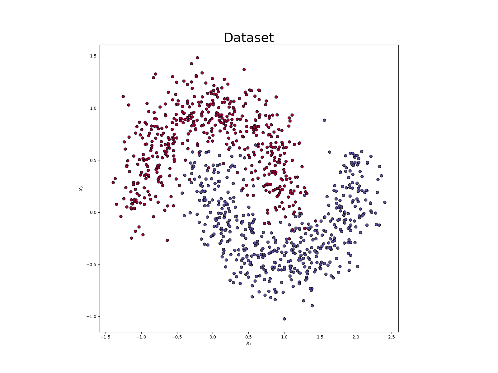_{^{The Moon dataset from the Sklearn library}}

We will train the model for 200 epochs. We also define some lists to store the accuracy and loss during the training.

acc_history = []
loss_history = []
N_EPOCHS = 200

We define some plot functions.

GRID_X_START = -1.5
GRID_X_END = 2.5
GRID_Y_START = -1.5
GRID_Y_END = 2

grid = np.mgrid[GRID_X_START:GRID_X_END:100j, GRID_Y_START:GRID_Y_END:100j]
grid_2d = grid.reshape(2, -1).T
XX, YY = grid
fs = 20

def make_plot(X, y, epoch, XX, YY, preds):
    plt.figure(figsize=(18, 12))
    axes = plt.gca()
    axes.set_xlabel('$X_1$', fontsize=fs)
    axes.set_ylabel('$X_2$', fontsize=fs)
    plt.title("Epoch # : {:05}".format(epoch), fontsize=30)
    CT = plt.contourf(XX, YY, preds.reshape(XX.shape), 25, alpha = 1, cmap=cm.Spectral)
    CS = plt.contour(XX, YY, preds.reshape(XX.shape), levels=[.5], cmap="Greys", vmin=0, vmax=.6, linestyles='dashed', linewidths=2)
    CS.collections[0].set_label("Decision boundary at 0.5")
    plt.scatter(X[:, 0], X[:, 1], c=y.ravel(), s=80, cmap=plt.cm.Spectral, edgecolors='black', label='Test data')
    cbar = plt.colorbar(CT, ticks=[0, 0.5, 1])
    cbar.ax.tick_params(labelsize=15)
    cbar.set_label(label='Classification probabilities',size=fs, rotation=270, labelpad=20)
    axes.set_xlim(XX.min(), XX.max())
    axes.set_ylim(YY.min(), YY.max())
    axes.set_xticks(())
    axes.set_yticks(())
    plt.legend(fontsize=20, loc='upper left')
    plt.tight_layout()
    plt.savefig("./plots_keras/keras_model_{:05}.png".format(epoch))
    plt.close()

def loss_acc(logs, epoch):
    acc_history.append(logs['accuracy'])
    loss_history.append(logs['loss'])
    plt.figure(figsize=(12, 8))
    plt.plot(acc_history, '-x')
    plt.plot(loss_history, '-o')
    plt.title('Epoch # : {:05}'.format(epoch), fontsize=30)
    plt.ylabel('Accuracy - Loss', fontsize=fs)
    plt.xlabel('Epoch #', fontsize=fs)
    plt.xlim([0, N_EPOCHS])
    plt.legend(['accuracy', 'loss'], loc='upper left', fontsize=12)
    plt.tight_layout()
    plt.savefig("./plots_keras/loss_acc_{:05}.png".format(epoch))
    plt.close()

def callback_plot(epoch, logs):
    """ Callback function that will run on every epoch """
    prediction_probs = model.predict(grid_2d, batch_size=32, verbose=0)
    make_plot(X_test, y_test, epoch, XX=XX, YY=YY, preds=prediction_probs)
    loss_acc(logs, epoch)

testmodelcb = keras.callbacks.LambdaCallback(on_epoch_end=callback_plot)

We define the network as follows with Keras.

model = Sequential()
model.add(Dense(25, input_dim=2,activation='relu'))
model.add(Dense(50, activation='relu'))
model.add(Dense(50, activation='relu'))
model.add(Dense(25, activation='relu'))
model.add(Dense(1, activation='sigmoid'))
model.compile(loss='binary_crossentropy', optimizer="sgd", metrics=['accuracy'])

We train the model.

history = model.fit(X_train, y_train, epochs=N_EPOCHS, verbose=0, callbacks=[testmodelcb])
prediction_probs = model.predict(grid_2d, batch_size=32, verbose=0)

Finally we test the model on the test set.

score = model.evaluate(X_test, y_test, verbose=0)
print('Test loss: {:.2f}'.format(score[0]))
print('Test accuracy: {:.2f}'.format(score[1]))

Y_test_hat = np.argmax(model.predict(X_test), axis=1)
acc_test = accuracy_score(y_test, Y_test_hat)
print("Test accuracy: {:.2f}".format(acc_test))

You can find the code on my Github.

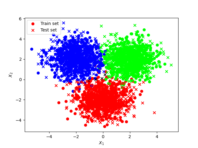
Comparison with Numpy

It is possible to implement the same network in Numpy, however the code is about 300 lines long vs only 100 lines for Keras.

We can plot the evolution of the cost function and the accuracy with the number of epochs for the Keras and Numpy implementation.

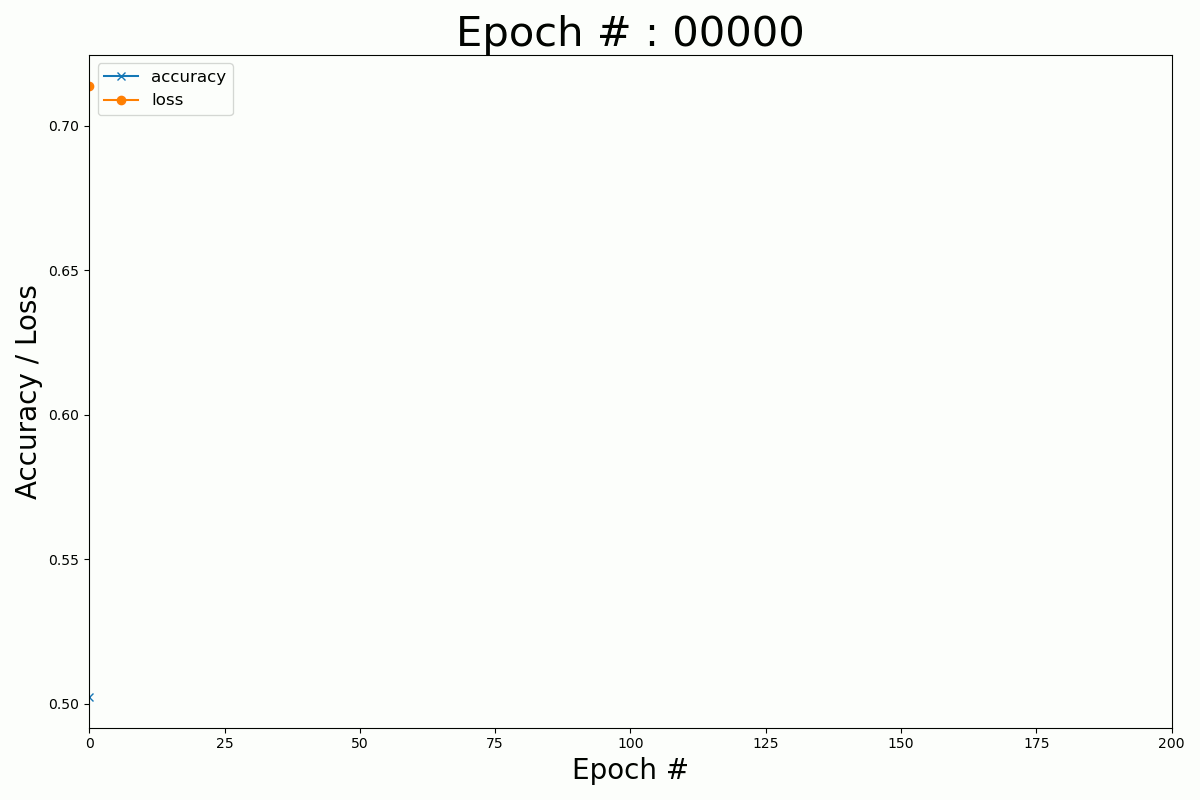_^Keras

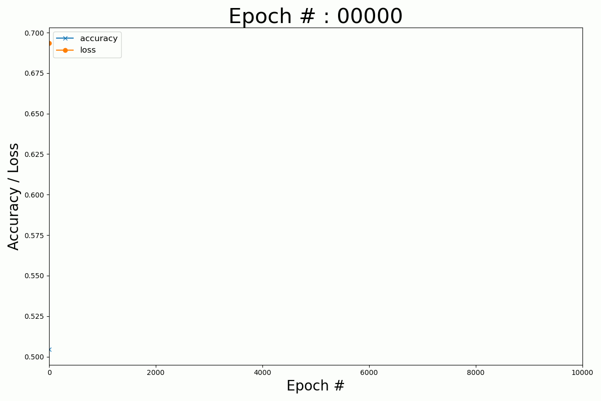_^Numpy

Here is a visualisation of the network classification probabilities, decision boundary, and test set for both the Keras and Numpy implementation.

_^Keras

_^Numpy

Conclusion

Keras is an user-friendly library for implementing neural network. In this post, we used Keras for binary classification of a non-linearly separable dataset.